The Real Capacitor: Non-Idealities, Impedance, and the Equivalent Circuit

2.1 When the ideal capacitor meets the bench

The foundational volume built an idealisation: two conductors, a farad or two of capacitance, a clean relationship Q = CV, and a reactance that falls smoothly forever as frequency rises. That capacitor is a fiction. It is a useful fiction — most of circuit design proceeds by pretending it is true — but it is a fiction, and the gap between it and the object soldered to the board is where the interesting engineering lives.

The real device is a wound roll or a fired stack of ceramic, connected to the outside world by metal that has resistance, wrapped in leads and terminations that have inductance, filled with a dielectric that stores energy imperfectly and lets a trickle of current leak straight through. Below a few kilohertz none of that matters much and the fiction holds. Above a few megahertz the fiction breaks so completely that a “bypass capacitor” stops being a capacitor at all and starts behaving as an inductor. In a switching power supply the difference between two 470 µF parts that measure identically on a cheap meter — one with 0.02 Ω of internal resistance, one with 2 Ω — is the difference between a supply that runs cool and one that cooks itself to death.

This volume replaces the ideal C with the model an engineer actually reasons about: a capacitance in series with a resistance and an inductance, shunted by a leakage path, its dielectric described not by a single number but by a complex, frequency-dependent one. The two signature pictures — the equivalent circuit and the impedance-versus-frequency curve — are worth committing to memory. Everything else in the passive-components world hangs off them.

2.2 The dielectric, told honestly: polarization mechanisms

The foundational volume said the dielectric raises capacitance by a factor εr, the relative permittivity, and left it there. To understand why one ceramic is rock-stable and another loses half its value in your hand, the mechanism behind that number has to come out.

Permittivity is a measure of how strongly a material polarizes — how much its internal charge separates and lines up — when an electric field is applied. That polarization is what lets the plates hold more charge at a given voltage. But polarization is not one thing. It is the sum of several distinct physical processes, each with its own sluggishness, and each drops out of the picture as the field is asked to reverse faster and faster.

• Electronic polarization is the electron cloud of every atom shifting slightly against its nucleus. It is nearly instantaneous — it keeps up into the ultraviolet, around 10¹⁵ Hz — and it is present in every material, even a vacuum-like gas. It contributes a small, extremely stable permittivity.
• Ionic (atomic) polarization is the displacement of positive ions relative to negative ions in a bonded lattice — the sodium and chlorine in table salt leaning apart. It responds up into the infrared, roughly 10¹²–10¹³ Hz, and adds more permittivity in ionic solids.
• Dipolar (orientational) polarization is the physical rotation of molecules that carry a built-in electric dipole, like water, twisting to align with the field. Rotating a whole molecule is slow and viscous; this mechanism runs out of breath somewhere between kilohertz and gigahertz depending on the material and its temperature. It can contribute enormous permittivity while it lasts.
• Interfacial (space-charge) polarization is charge piling up at internal boundaries — grain edges, electrode interfaces, impurities. It is the slowest of all, relevant from sub-hertz to kilohertz, and is the usual culprit behind large low-frequency permittivity and its associated losses.

The picture below is the master diagram of dielectric physics: as frequency climbs, one mechanism after another can no longer follow the field and switches off. The stored permittivity ε′ steps down in a staircase, and at each step the material dissipates energy — a loss peak — because the polarization is now lagging the field and dragging against it.

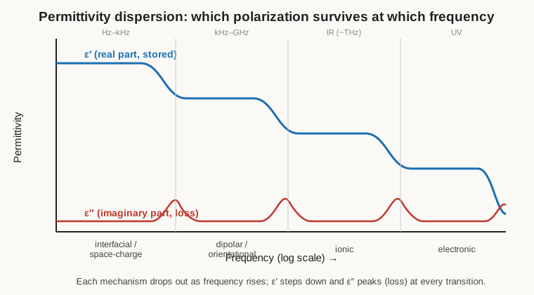
This one diagram forward-explains the entire ceramic volume. The ultra-stable Class I ceramics (the C0G/NP0 parts) lean almost entirely on electronic and ionic polarization — the fast, temperature-insensitive mechanisms — which is why their capacitance barely moves with temperature or frequency and why they carry so little loss. The high-value Class II ceramics (X7R, X5R, and the notorious Y5V) rely on ferroelectric dipolar polarization in barium-titanate grains, which is why they pack enormous capacitance into a tiny package and also why that capacitance sags with temperature, ages with time, and collapses under DC bias. The ceramic volume covers that DC-bias loss in detail; the mechanism table above is why it exists at all.

2.2.1 Complex permittivity: ε = ε′ − jε″

Because the polarization lags the field, permittivity is properly written as a complex number:

ε = ε′ − jε″

The real part ε′ is the energy the dielectric stores and gives back each cycle — the “capacitance” part. The imaginary part ε″ is the energy it fails to give back, converted to heat — the “loss” part. Their ratio is the material’s intrinsic loss tangent:

tan δ = ε″ / ε′

This is the same tan δ that appears on a capacitor datasheet as dissipation factor, seen from the material’s side rather than the circuit’s. A perfect dielectric has ε″ = 0; a lossy one, near one of those loss peaks, can dissipate a serious fraction of the energy that passes through it. And because ε′ and ε″ both depend on frequency and temperature, so does everything measured at the terminals. The single number “εr = 2000” printed in a textbook is shorthand for “at some particular frequency and temperature the real part happened to be 2000.”

2.3 The equivalent circuit

Take that non-ideal dielectric, wrap it in real metal, and the whole device collapses — for engineering purposes — into four lumped elements.

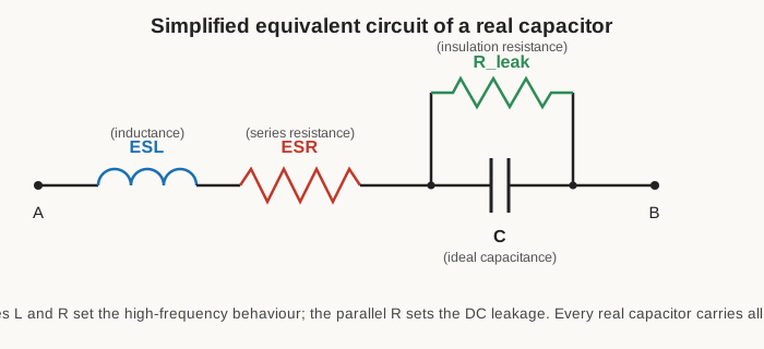
• C — the ideal capacitance, the thing the part is sold as.
• ESR — equivalent series resistance — a single resistor that lumps together every dissipative loss in series with the plates: the resistance of the electrodes, the terminations, and the leads, plus the dielectric loss (ε″) referred to the terminals. It is what turns ripple current into heat.
• ESL — equivalent series inductance — a single inductor representing the magnetic field of current flowing through the electrodes, terminations, and leads. It is what makes a capacitor stop working at high frequency.
• R_leak — insulation resistance — a large resistor in parallel with C, the path by which a charged capacitor slowly discharges itself through its own imperfect dielectric.

More elaborate models exist — dielectric absorption is often drawn as a ladder of extra R-C pairs hung across C, and ESR is really frequency-dependent rather than a fixed resistor — but this four-element picture answers the great majority of bench questions. The rest of this volume is essentially a tour of what each parasitic costs.

2.4 ESR: the resistance that heats

Equivalent series resistance is the parameter that quietly decides whether a design works. It has two physical sources. The first is honest ohmic resistance: the thin metal electrodes, the crimps and welds, the leads. The second is the dielectric loss — the ε″ term — mathematically transformed into a resistance in series with the plates. At low frequency, dielectric loss usually dominates ESR; at high frequency, the metal resistance dominates. The result is that ESR is not a constant. It typically falls as frequency rises (dielectric loss thinning out), flattens toward a metallic floor, and it changes with temperature — dramatically so in wet aluminium electrolytics, whose electrolyte becomes more resistive as it gets cold, so their ESR can multiply several-fold at −40 °C.

Why does it matter? Two reasons, both about heat and both about high-current jobs.

First, ripple heating. Any AC current forced through the capacitor dissipates power in the ESR at P = I²·ESR. In a switching supply’s output capacitor, that ripple current can be amperes, and even a fraction of an ohm becomes a meaningful number of watts deposited inside a small can. That heat is why electrolytics wear out and is treated as a hard rating in its own right, below.

Second, decoupling effectiveness. A bypass capacitor’s job is to be a low impedance at the frequency of interest; its ESR sets the floor of that impedance. You cannot get below the ESR no matter how much capacitance you add. For a processor pulling sharp current transients, milliohms of ESR is the difference between a clean supply rail and one that sags on every clock edge.

The spread of ESR across families is the whole story of why different capacitors exist:

Table 1 — The spread of ESR across families is the whole story of why different capacitors exist

Family	Typical ESR (order of magnitude)	Comment
MLCC ceramic	single-digit to tens of mΩ	The reason ceramics dominate modern decoupling
Film (PP/PET)	milliohms to tenths of an ohm	Low loss, but bulky per farad
Polymer aluminium / polymer tantalum	~5–30 mΩ	Solid electrolyte, near-ceramic ESR at high capacitance
Wet aluminium electrolytic	tenths of an ohm to several Ω	High, and strongly temperature-dependent
Solid tantalum (MnO₂)	tenths of an ohm to a few Ω	Moderate; polymer versions much lower

That two-order-of-magnitude gap between a ceramic and a wet electrolytic is why a switching-supply designer parallels a big electrolytic (bulk energy storage, high ESR, cheap farads) with a clutch of small ceramics (low ESR, fast) — each doing the job the other cannot.

2.5 Dissipation factor, loss angle, and Q

The dielectric people speak of tan δ; the circuit people speak of ESR; the RF people speak of Q. They are three views of the same loss.

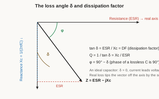
Picture the capacitor’s impedance as a vector in the complex plane. An ideal capacitor’s impedance is purely imaginary — the current leads the voltage by exactly 90°, and no energy is lost. A real capacitor has that small series resistance, so the impedance vector tips off the pure-reactance axis by a small angle δ, the loss angle.

From the geometry:

DF = tan δ = ESR / Xc where Xc = 1 / (2πfC)

DF, the dissipation factor, is just tan δ expressed as a number (often a percentage). It is the fraction of energy lost per cycle relative to energy stored. Rearranging gives the single most useful conversion in this whole volume, the bridge between the datasheet’s DF and the number you actually want:

ESR = DF / (2πfC)

That is how a datasheet quoting “DF = 2.5% at 120 Hz” for an electrolytic becomes an ESR in ohms, or how a C0G’s “DF ≤ 0.1% at 1 MHz” becomes milliohms. The catch is that both DF and the f in the formula have to be quoted at the same frequency; an electrolytic’s DF at 120 Hz tells you almost nothing about its ESR at 100 kHz.

The quality factor Q is simply the reciprocal:

Q = 1 / DF = 1 / tan δ = Xc / ESR

High Q means low loss — the phrase “high-Q capacitor” for an RF tuning part means the same thing as “low DF.” A C0G ceramic or a silver-mica cap can have a Q in the thousands; a general-purpose electrolytic has a Q below 10 at its rated test frequency.

Typical dissipation factors, useful as sanity checks:

Table 2 — Typical dissipation factors, useful as sanity checks

Family	Typical DF (tan δ)	Test frequency
C0G / NP0 ceramic	≤ 0.1 %	1 MHz
Polypropylene / polystyrene film	0.02–0.1 %	1 kHz
X7R / X5R ceramic	1–3 %	1 kHz
Polyester (PET) film	0.3–1 %	1 kHz
Solid tantalum	2–10 %	120 Hz
Aluminium electrolytic	5–20 %	120 Hz

2.6 Impedance versus frequency: the signature curve

Assemble C, ESR, and ESL in series and ask what the magnitude of the impedance does across frequency. The reactances add as vectors, the resistance sits underneath, and the result is:

|Z| = √( ESR² + (Xc − XL)² ) where Xc = 1 / (2πfC) and XL = 2πfL

Plotted on log-log axes it makes the shape every hardware engineer should recognise on sight.

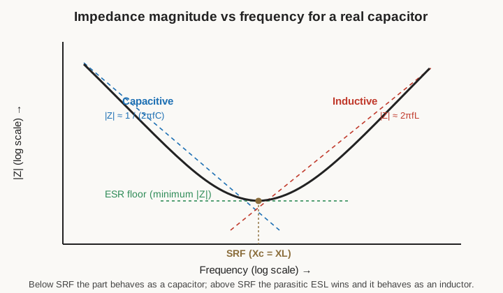
Read it left to right.

• The capacitive region. At low frequency Xc is large and XL is negligible, so |Z| ≈ 1/(2πfC) — a straight line falling at −20 dB per decade. Here the part behaves the way the foundational volume promised. More capacitance moves this line down.
• The minimum. As frequency rises, Xc falls and XL rises. At the self-resonant frequency (SRF) they are equal and opposite, Xc = XL, they cancel completely, and all that remains is the ESR. The impedance bottoms out at a floor equal to the ESR. This is the frequency at which the capacitor is most effective as a bypass — and it is a genuinely useful number, not just a curiosity.
• The inductive region. Above SRF, XL dominates and |Z| ≈ 2πfL — a line rising at +20 dB per decade. The device is now, electrically, an inductor. A 100 nF “decoupling capacitor” whose SRF is 15 MHz provides increasing impedance to a 100 MHz noise spike; it is doing the opposite of its job.

The self-resonant frequency itself is set by the ideal LC resonance of the internal capacitance and the ESL:

SRF = 1 / (2π √(L·C))

Two consequences follow immediately, and both drive real layout decisions.

Smaller packages resonate higher. ESL is dominated by the physical loop the current traces through the part and its mounting. A tiny 0402 chip has perhaps 0.3–0.5 nH of ESL; an 0805 around 0.5 nH; a 1206 roughly 1–2 nH; a leaded electrolytic, tens of nanohenries. Less inductance, higher SRF. That is why the same 100 nF value in a smaller case is the better high-frequency bypass, and why RF designers reach for the smallest package they can place. A representative ladder — the exact numbers depend on value and vendor, but the trend is universal:

Table 3 — Smaller packages resonate higher. ESL is dominated by the physical loop the current traces through the part and its mounting. A tiny 0402 chip has perhaps 0.3–0.5 nH of ESL; an 0805 around 0.5 nH; a 1206 roughly 1–2 nH; a leaded electrolytic, tens of nanohenries. Less inductance, higher SRF. That is why the same 100 nF value in a smaller case is the better high-frequency bypass, and why RF designers reach for the smallest package they can place. A representative ladder — the exact numbers depend on value and vendor, but the trend is universal

Part	Rough ESL	Rough SRF
0402 MLCC, ~1–10 nF	~0.4 nH	hundreds of MHz
0805 MLCC, 100 nF	~0.5 nH	~15–30 MHz
1206 MLCC, ~1 µF	~1–2 nH	a few MHz
Leaded aluminium electrolytic, 100s of µF	tens of nH	tens to low hundreds of kHz

Higher capacitance also resonates lower — bigger C pushes SRF down for the same ESL — which is why a bulk 10 µF part and a 100 nF part have their impedance minima at very different places. Designers exploit that by paralleling different values so that each covers a different band of the spectrum, keeping the combined impedance low across decades.

There is a trap in that trick, and it is worth stating plainly because it catches good engineers. When a large capacitor (already inductive above its SRF) is paralleled with a small one (still capacitive below its own SRF), there is a band between the two where one looks inductive and the other capacitive. They form a parallel LC tank, and at its resonance the combined impedance spikes upward — anti-resonance. Blindly stacking many values can create a picket fence of impedance peaks. The cure is to keep the value ratios modest (roughly a decade, not three), to use several of the same value rather than many different ones, and to lean on low-ESR parts, since ESR damps the anti-resonant peak.

A last, humbling point about ESL: much of it is not even inside the capacitor. The loop from the pad, through the via, down to the plane and back adds mounting inductance that frequently exceeds the part’s own ESL. A perfect 0.4 nH capacitor mounted on 2 nH of vias and traces resonates as if it were a 2.4 nH part. High-speed decoupling is won or lost in the layout, not the bill of materials.

2.7 Leakage, insulation resistance, and self-discharge

No dielectric is a perfect insulator. Apply a DC voltage and a small leakage current flows straight through, modelled by R_leak in parallel with the ideal capacitance. Left disconnected, a charged capacitor bleeds itself down through this path with a time constant τ = R_leak · C — the self-discharge time.

Because a bigger capacitor of a given technology has more electrode area (and therefore more leakage paths in parallel, lowering R_leak), manufacturers do not quote the insulation resistance directly. They quote the product R · C, in ohm-farads or, conventionally, megohm-microfarads (MΩ·µF). Divide the rated product by your capacitance to get the insulation resistance of your particular part, subject to an absolute ceiling (a datasheet reads “10⁵ MΩ·µF or 100 GΩ, whichever is less”).

Here is the elegant part, and it is a genuine engineer’s payoff: one megohm-microfarad is exactly one second. (10⁶ Ω × 10⁻⁶ F = 1 Ω·F = 1 s.) So the RC-product spec, read as a number, is the self-discharge time constant in seconds — no arithmetic required. That reframes the whole family comparison:

Table 4 — Here is the elegant part, and it is a genuine engineer's payoff: one megohm-microfarad is exactly one second. (10⁶ Ω × 10⁻⁶ F = 1 Ω·F = 1 s.) So the RC-product spec, read as a number, is the self-discharge time constant in seconds — no arithmetic required. That reframes the whole family comparison

Family	Typical RC product	Self-discharge τ
Polypropylene / C0G ceramic	10⁴–10⁵ MΩ·µF	hours to a day-plus
Polyester (PET) film	~10⁴ MΩ·µF	hours
X7R ceramic	~10³ MΩ·µF	~15 minutes
Aluminium electrolytic	— (spec’d as leakage current)	seconds to minutes

Aluminium electrolytics and tantalums leak far too much for the RC convention to be flattering, so their datasheets give a leakage current limit instead — typically a formula of the form I = K·C·V plus a floor, measured after a few minutes of applied rated voltage (the current is much higher at switch-on and settles as the oxide “heals”). A big electrolytic can leak milliamps; a good film cap, picoamps. That is exactly why a sample-and-hold, an integrator, or a long timing circuit is built around film or C0G and never around an electrolytic: you want the charge to stay put, and only the high-insulation-resistance dielectrics oblige.

2.8 Dielectric absorption: the charge that comes back

Leakage is charge trickling away. Dielectric absorption is charge that was already thought gone coming back, and it surprises people the first time they meet it.

Charge a capacitor to a healthy voltage, hold it a while, then short the terminals briefly to dump the charge to zero. Remove the short and leave the terminals open. Over the following seconds to minutes, a voltage reappears at the terminals — a few millivolts to a few percent of the original, climbing and then slowly fading. The capacitor seems to remember. Bench slang calls it soakage or “battery action.”

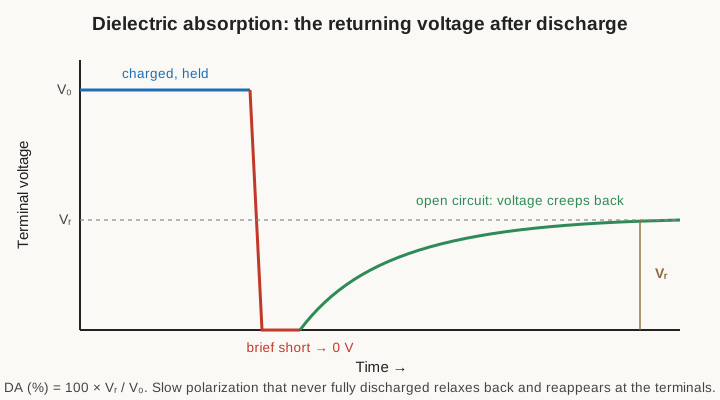
The mechanism is the slow polarization from the earlier diagram. The fast electronic and ionic polarizations discharge instantly during the short; the slow dipolar and interfacial polarizations do not — some of that internal charge separation is still relaxing when the short is removed. As it relaxes, it re-establishes a field across the plates, and a voltage appears. Dielectric absorption is the time-domain fingerprint of the same lossy, laggy polarization that shows up as ε″ in the frequency domain.

It is quantified as DA (%) = 100 × V_r / V₀, the returning voltage as a fraction of the original charge voltage, and it tracks the dielectric almost perfectly:

Table 5 — It is quantified as DA (%) = 100 × Vr / V₀, the returning voltage as a fraction of the original charge voltage, and it tracks the dielectric almost perfectly

Dielectric	Typical DA
Polystyrene, polypropylene, Teflon (PTFE)	0.01–0.05 %
Polyester (PET) film	0.2–0.5 %
C0G / NP0 ceramic	< 0.1 %
X7R ceramic	~1–2.5 %
Aluminium / tantalum electrolytic	10 % or more

For a decoupling capacitor, DA is irrelevant. For precision analog it is a quiet menace. In a sample-and-hold, the returning voltage corrupts the held value between samples. In a precision integrator or an analog computer, it introduces a memory of past inputs — the circuit’s own hysteresis. In a high-resolution ADC’s sampling capacitor, it costs you bits. This is precisely why the classic advice for those jobs is polypropylene, polystyrene, or Teflon — and never the high-K ceramics or electrolytics that are otherwise so convenient. The measurement volume returns to how DA is actually tested (the standardised charge/short/soak intervals matter, since DA is time-dependent).

2.9 Voltage: working, surge, breakdown, and the culture of derating

Every capacitor carries a rated (working) voltage — the maximum DC it is designed to sustain continuously. Above it sits a higher surge voltage, a transient limit the part can tolerate briefly and occasionally (electrolytics typically rate surge around 10–15 % above working). Above that lies breakdown, where the dielectric fails outright — for a film or ceramic, a punch-through short; for an electrolytic, a vent; for a tantalum, potentially ignition.

Experienced engineers rarely run a capacitor anywhere near its rating, and the reasons differ by family — this is derating culture, and it is not superstition.

• Ceramics (Class II). Two problems compound. First, reliability: ceramic failure rate climbs steeply with applied voltage, so running well below rated buys orders of magnitude in lifetime. Second, and unique to Class II, is DC-bias capacitance loss — an X7R or X5R can lose 50–80 % of its rated capacitance when operated near its rated voltage, because the DC field saturates the ferroelectric polarization. A “10 µF 6.3 V” X5R sitting on a 5 V rail might deliver 3 µF. The habit of running MLCCs at half their rated voltage (or less) is as much about keeping the capacitance as about reliability. The ceramic volume dwells on this at length.
• Tantalum. The solid-tantalum surge-failure mechanism is violent — a local defect can trigger a self-sustaining short that ignites. The long-standing rule is a 2:1 voltage derating (run at 50 % of rated, or less) on low-impedance rails, which dramatically cuts the surge-failure rate. The tantalum volume covers the mechanism.
• Aluminium electrolytic. Less dramatic, but running at ~80 % of rated and keeping ripple within spec extends the wear-out life. Leaving one unpowered for years lets its oxide degrade, hence “reforming” — also a later-volume topic.
• Film. The most forgiving, thanks to self-healing in metallized types (a fault vaporises the thin metal and clears itself), but AC and pulse duty derates the DC rating hard, since dV/dt drives real current.

The through-line: rated voltage is a ceiling, not an operating point. Prudent designs sit comfortably below it.

2.10 Temperature: two entirely different roles

“Temperature rating” on a capacitor conflates two separate ideas, and confusing them causes real errors.

The first is the maximum operating temperature — a survival limit, the classic 85 °C / 105 °C / 125 °C (and 150 °C for specialty parts) classes. Exceed it and the part degrades or fails; for electrolytics, every 10 °C over accelerates the wear-out dramatically (the Arrhenius rule of thumb — life roughly halving per 10 °C — gets its own treatment in the electrolytic volume).

The second is the temperature coefficient — how much the capacitance value drifts with temperature, quoted in ppm/°C for stable dielectrics or as a percentage tolerance band over a temperature range for the high-K ones. A C0G ceramic is specified at 0 ± 30 ppm/°C — flat as a table. An X7R is specified to stay within ±15 % of its 25 °C value from −55 to +125 °C, which is a survival promise, not a stability one. The EIA letter-number codes that encode all this (the X7R, Y5V, C0G alphabet) are decoded in the ceramic volume; the point here is that a “125 °C capacitor” tells you it survives to 125 °C, not that its value holds there.

2.11 Ripple current and self-heating: a rating you can exceed

ESR plus AC current equals heat, and heat is the thing that kills capacitors. The power dissipated inside the part is P = I_rms² · ESR, deposited in a small volume with limited ability to shed it. Push too much ripple current and the core temperature climbs past the rating, and the part ages fast or fails.

For this reason ripple current is a hard, published rating, especially for electrolytics and film caps in power supplies — a maximum I_rms (at a stated frequency and ambient temperature) that keeps the internal rise within bounds. It is not a soft guideline; exceed it and the datasheet’s endurance numbers no longer apply. Because ESR falls with frequency, the allowable ripple current usually rises with frequency, and datasheets provide multiplier tables to translate the 120 Hz rating to 100 kHz. This rating is also why the low-ESR of ceramics and polymer electrolytics is such a prize: less ESR means less self-heating for the same ripple, which means either a cooler part or a smaller one. The lifetime and wear-out consequences of running near the ripple limit are the subject of the electrolytic volume.

2.12 Aging

A quieter non-ideality: some dielectrics age, losing capacitance slowly and predictably with time after manufacture. Class II ferroelectric ceramics age at a roughly constant percentage loss per decade of hours — a few percent per decade-hour is typical — as the crystal structure relaxes toward a lower-energy state. Heating the part above its Curie point (“de-aging”) resets the clock, and the process begins again. C0G ceramics and film do not meaningfully age. Aging matters when a capacitance value is specified tightly; the ceramic volume gives the numbers. Distinct from aging is wear-out — the electrolyte-drying end-of-life of aluminium electrolytics — which is a consumable-lifespan story told in its own volume.

2.13 Reading a real datasheet

Everything above lands on one or two pages of a manufacturer datasheet, and the parameters now have names and meanings.

At the top sit capacitance, its tolerance (±10 %, ±20 %, the K and M codes), and the rated voltage — the ideal-C headline and its ceiling. Nearby is the temperature characteristic — a C0G/X7R code for ceramics, a ppm/°C or ±% figure for others — which is the temperature coefficient, not the survival temperature; the survival temperature is the separate operating temperature range (−55 to +125 °C and friends).

Then the non-idealities. Dissipation factor or tan δ appears with its test frequency (120 Hz for electrolytics, 1 kHz or 1 MHz for ceramics and film) — convert it to ESR via ESR = DF/(2πfC), or read ESR directly if the part is a low-ESR type that quotes it. Ripple current shows up for power parts, with frequency and temperature multiplier tables. Insulation resistance appears either as an MΩ·µF product (read it as the self-discharge time in seconds) or, for electrolytics, as a leakage-current limit and its measuring conditions. ESL or a plotted impedance-versus-frequency curve appears on parts sold for decoupling — and that curve, with its falling capacitive slope, its ESR-floored minimum at SRF, and its rising inductive tail, is Figure 4 drawn by the vendor for that exact part number.

Learn to read those three curves — impedance versus frequency, ESR versus frequency, and (for Class II ceramics) capacitance versus DC bias — and the datasheet stops being a table of disconnected numbers and becomes a portrait of the equivalent circuit for one specific part. On the bench, the same portrait is drawn by an LCR meter, which measures capacitance, DF, and ESR at chosen frequencies, and by a dedicated ESR meter for in-circuit electrolytic checks — the instruments the measurement volume covers in full.

2.14 The real capacitor, in one paragraph

The ideal capacitor stores charge and nothing else. The real one carries a resistance that heats it, an inductance that turns it into an inductor above its self-resonant frequency, a leakage path that discharges it, and a dielectric whose polarization lags, loses, sags with bias, drifts with temperature, ages with time, and hands back a ghost of charge after it is emptied. None of this makes the ideal model wrong — it makes it incomplete, and the incompleteness is bounded and knowable. Every parameter has a home in the four-element equivalent circuit, a home on the datasheet, and a home on the impedance-versus-frequency curve. The family volumes that follow — ceramic, film, aluminium, tantalum, and the rest — are, at bottom, the story of how each construction trades these non-idealities against one another, and the measurement volume is the story of how to see them for yourself.