The Real Inductor: Losses, Self-Resonance, and Saturation

2.1 When the ideal inductor meets the bench

The foundational volume built an idealisation: a coil of wire whose only property is inductance L, whose reactance X_L = 2πfL rises cleanly and forever with frequency, and which stores energy in its magnetic field and gives every joule back. That inductor is a fiction. It is a useful fiction — a great deal of circuit design proceeds by pretending it is true — but it is a fiction, and the distance between it and the wound object clamped in a test fixture is exactly where the interesting engineering lives.

The real device is a length of copper, wrapped many times around a core or around air, and the copper has resistance. The turns sit next to one another, and any two conductors at different voltages form a small capacitor, so the coil quietly builds a capacitor into itself. If there is a magnetic core, that core dissipates energy every time the field reverses, and it has a ceiling: push enough current through the winding and the core simply runs out of magnetism, at which point the inductance collapses. None of this appears in L = μ₀μ_rN²A/ℓ.

Two consequences dominate everything that follows. First, a real inductor works as an inductor only over a band of frequencies — too low and the copper resistance swamps it; too high and its own self-capacitance turns it into a capacitor. Second, a real inductor works only up to a current — beyond that the core saturates and the part is no longer the value stamped on it. Self-resonance and saturation are the two effects every engineer must carry in their head, and this volume is largely a tour of them and of the parasitic elements that produce them. As with the companion capacitor dive, two pictures — the equivalent circuit and the impedance-versus-frequency curve — are worth committing to memory.

2.2 The equivalent circuit, first

Everything the bench sees collapses, for engineering purposes, into a handful of lumped elements hung around the ideal L.

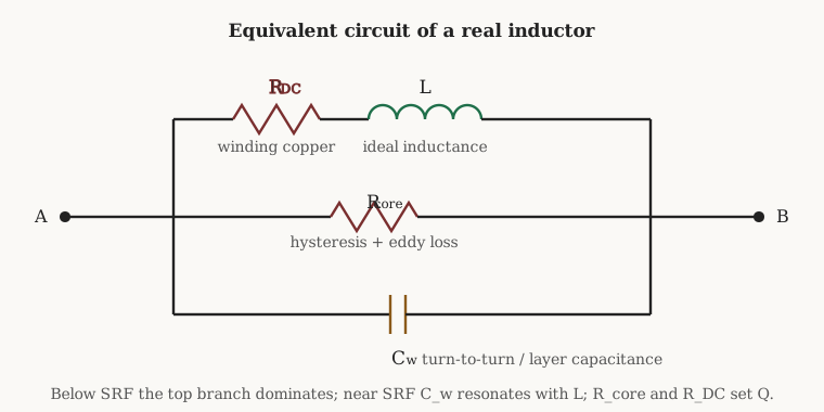
Read left to right. R_DC is the plain copper resistance of the wire, in series with the coil because the current must flow through the whole winding to reach the far terminal. L is the ideal inductance the part is sold as. Shunting that series branch is C_w, the winding’s self-capacitance, which offers the current an alternative path around the inductance — a path that becomes irresistible at high frequency. Also in parallel sits R_core, a resistance that stands in for the energy the magnetic core throws away as heat each cycle; unlike the copper resistance it is not really a fixed ohmic value but a bookkeeping device that rises with frequency and flux.

More elaborate models exist — R_core is sometimes split into separate hysteresis and eddy-current elements, R_DC is really frequency-dependent once skin effect bites, and C_w is a lumped stand-in for a distributed capacitance smeared along the whole winding — but this four-element picture answers the large majority of bench questions. The remainder of this volume walks each element in turn and shows what it costs.

2.3 DC resistance: the copper that heats

Start with the least glamorous parasitic and arguably the most consequential. The winding is copper, copper has a resistivity of about 1.68 × 10⁻⁸ Ω·m, and a coil is simply a long thin conductor coiled up. Its DC resistance — universally abbreviated DCR on datasheets — is set by the same schoolroom relation as any wire: resistance rises with length and falls with cross-sectional area. Put more turns on, or wind them on a bigger former so each turn is longer, and DCR climbs in proportion to the wire paid out. Move to a fatter gauge and DCR falls as the square of the diameter. The wire volume covers gauge, the AWG scale, and current ratings in detail; here the point is only that DCR is a direct, unavoidable consequence of the turns and the gauge, and the two design goals — high inductance (many turns) and low resistance (few, fat turns) — pull against each other.

DCR matters for three reasons. The first is heat: a current I flowing through the winding dissipates *I²·*DCR watts as copper loss, and that power warms the part. In a switching-regulator inductor carrying several amps, DCR is often the single largest loss in the whole magnetic component, and it is why a power inductor’s datasheet leads with milliohms. The second is Q, the quality factor treated below: DCR is the dominant series loss at low and moderate frequencies, and every milliohm of it drags Q down. The third is a plain voltage drop — a filter choke passing DC develops *I·*DCR volts across itself, wasted headroom in a low-dropout supply and a self-heating term besides.

One subtlety that trips up the unwary: DCR is not constant with temperature. Copper’s resistance rises about 0.39 % for every degree Celsius, so a winding that measures 100 mΩ at 25 °C reads roughly 130 mΩ once self-heating has taken it to 100 °C. Copper loss therefore has a mild thermal-runaway flavour — more current, more heat, more resistance, more heat — though in practice it is gentle and self-limiting rather than destructive.

2.3.1 Copper loss versus core loss

It helps to divide an inductor’s total loss into two buckets that behave completely differently. Copper loss (also winding loss) is the *I²·*R heating in the wire; at DC and low frequency it is essentially all DCR, and it depends on the current. Core loss is the energy the magnetic material dissipates, and it depends on the flux swing and the frequency, not directly on the load current. A choke carrying a large DC current with only a little ripple is copper-loss dominated; a transformer or an inductor driven with a large AC swing at high frequency can be core-loss dominated. Total loss is the sum, the two respond to different variables, and separating them is the first move in diagnosing why a magnetic part is running hot. Core loss gets its own section below, and the full treatment in the core-materials volume.

2.4 Winding capacitance: a capacitor hiding in the coil

Wind a hundred turns of enamelled wire onto a former and something inconvenient happens for free: every pair of adjacent turns, sitting a wire-diameter apart at slightly different potentials, forms a tiny capacitor, and every layer wound over another layer faces the layer beneath across the enamel like the plates of a still larger one. Summed over the whole coil these add up to a single effective winding capacitance, C_w, that appears in parallel with the inductance. It is usually small — anywhere from a fraction of a picofarad for a tidy single-layer air-core coil to tens or even hundreds of picofarads for a large multilayer choke — but small is not zero, and at high frequency a few picofarads is all it takes.

The geometry of the winding sets C_w, which is precisely why winding technique is a subject in its own right rather than an afterthought. The worst case is a multilayer coil wound back and forth in neat layers: the wire at the end of one layer lies directly over the wire at the start of the next, so turns many volts apart end up physically adjacent, and the layer-to-layer capacitance is large. Three classic dodges reduce it. Single-layer solenoids keep every turn near its neighbours in voltage and put no layer over another, so C_w is minimal. Space-winding — leaving a gap between turns — cuts the turn-to-turn capacitance further. And the universal or honeycomb winding used in old radio coils lays the wire on at a steep, constantly reversing angle so that adjacent turns cross rather than run parallel, minimising the area and dwell over which two conductors face each other. The winding-technique volume covers all three in the depth the subject deserves; the takeaway here is that C_w is not a fixed property of a coil’s inductance but a thing the winder controls.

2.5 Self-resonant frequency: where the inductor stops being one

Put the inductance L in parallel with its own winding capacitance C_w and the result is a resonant tank — the same LC resonance that makes a tuned circuit, except here it is unintentional and built into the part. The frequency at which it resonates is the inductor’s self-resonant frequency, or SRF:

f_SRF = 1 / (2π√(L·C_w))

Below the SRF the inductive reactance dominates and the part behaves as advertised: impedance rises with frequency. At the SRF the inductive reactance and the capacitive reactance are equal and opposite; they cancel, and what is left is a very high impedance limited only by the coil’s losses — a parallel-resonant peak. Above the SRF the capacitive reactance wins, the impedance falls with rising frequency, and the “inductor” now behaves for all the world like a capacitor. It is worse than useless above its SRF; it is actively the wrong component.

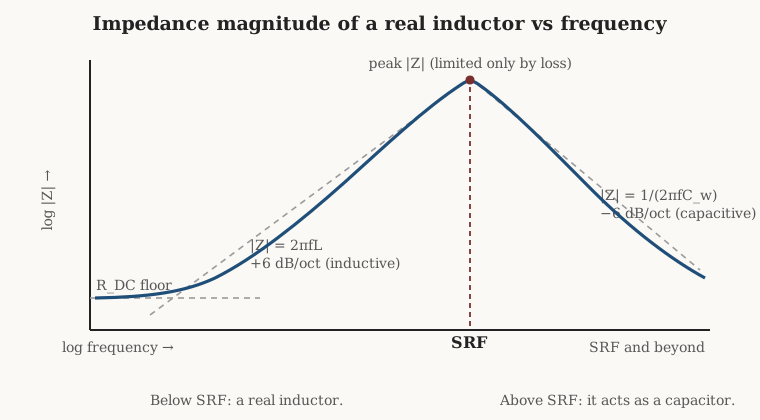
That inverted-V is the signature plot of a real inductor, and it carries two design rules. First, keep the operating frequency comfortably below the SRF — a common rule of thumb is to stay below roughly a tenth of it, where the reactance is still cleanly inductive and C_w has not yet begun to bend the curve. Second, remember that SRF and inductance trade against each other. A larger inductance means more turns, more turns mean more winding capacitance, and more of both lowers the SRF; so high-value inductors self-resonate low and high-frequency inductors are necessarily small. A 10 µH power inductor might self-resonate around 20–50 MHz; a 100 nH RF chip inductor might not resonate until well past a gigahertz. The manufacturer’s job, and the winder’s, is to push the SRF as far above the intended operating band as construction allows — which is one more reason low-capacitance winding geometries exist.

2.6 Quality factor Q: energy kept versus energy lost

The quality factor Q measures how close a real inductor comes to the lossless ideal. Formally it is the ratio of the inductive reactance to the total series loss resistance:

Q = X_L / R_series = 2πfL / R_series

Equivalently, and more physically, Q is 2π times the energy stored in the magnetic field divided by the energy dissipated per cycle. A Q of 100 means the coil returns a hundred times as much energy to the circuit each cycle as it wastes; a Q of 5 means it is throwing away a fifth of what it stores. R_series here is the effective series resistance — not just DCR, but DCR plus the AC copper losses from skin and proximity effect plus the core loss, all referred to a single resistance in series with L. That distinction is what makes Q interesting, because R_series grows with frequency while X_L also grows with frequency, and the two race.

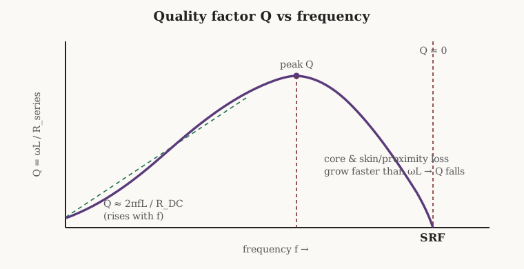
At low frequency R_series is essentially the fixed DCR, so Q climbs almost linearly with frequency as 2πfL/DCR. As frequency rises the effective resistance begins to swell — skin effect thins the usable copper, proximity effect crowds the current, and core loss mounts — and eventually R_series grows faster than the reactance. Q reaches a broad peak, often somewhere in the coil’s intended operating band, and then rolls off, falling all the way to zero at the SRF (where the net reactance vanishes, so there is nothing to divide by the loss). The location and height of that peak is a headline number for RF coils.

Whether high Q is a virtue depends entirely on the job. In a tuned circuit or filter, Q sets the sharpness of the resonance and the insertion loss: a high-Q inductor gives a narrow, selective peak and a low-loss filter, which is why RF coils are wound with fat wire, on low-loss cores or none, in low-capacitance geometries, chasing Q values from the low hundreds up toward four hundred for the best air-core work. In a damping or EMI-suppression role the opposite is wanted: a ferrite bead or a common-mode choke is supposed to be lossy, deliberately built from high-loss ferrite so that it converts unwanted high-frequency energy into heat rather than resonating with it. There the low Q is the feature. Power inductors sit in between, with modest Q, because their designers are spending the copper budget on low DCR and high saturation current rather than on a sharp resonance.

2.7 Core losses: hysteresis and eddy currents

Whenever a magnetic core carries an alternating flux it dissipates energy, by two distinct mechanisms, and both are introduced here and treated fully in the core-materials volume.

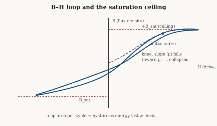
Hysteresis loss is the energy spent dragging the core’s magnetic domains back and forth. A ferromagnetic material does not magnetise and demagnetise along the same path; plot flux density B against magnetising force H and the trace forms a loop rather than a line, and the area enclosed by that loop is energy lost as heat on every cycle. Wider loop, more loss. Multiply by the number of cycles per second and hysteresis loss rises in proportion to frequency and steeply with the flux swing.

Eddy-current loss is different in origin. A changing magnetic field induces circulating currents inside the core material itself, by exactly the Faraday-law mechanism that makes the inductor work — and those induced currents flow through the core’s own resistance and dissipate power. Because the induced voltage rises with frequency, eddy loss climbs roughly as the square of frequency and as the square of flux, making it the villain at high frequency. The entire zoo of core constructions exists to fight it. Laminating an iron core — building it from thin varnished sheets rather than a solid block — breaks the wide eddy-current loops into many small ones and throttles the loss, which is why mains transformers are stacks of thin steel. Ferrites are ceramics with intrinsically high electrical resistivity, so eddy currents can barely flow at all, which is what lets them work up into the megahertz. Powdered-iron and other powder cores are built from insulated metal grains, each too small and too isolated to host a meaningful eddy loop. All of it is engineering against that f²B² term.

The practical upshot, and the reason core loss appears in this volume at all, is that it inflates the effective series resistance (the R_core of Figure 1), drags down Q, and heats the part independently of the load current. An empirical relation named for Charles Steinmetz captures the behaviour well enough for design: core loss per unit volume goes roughly as P_v = k·f^α·B^β, with the exponent α somewhere near 1 to 1.7 and β near 2 to 3 for typical power ferrites — numbers the core volume unpacks with real material data. The lesson to carry forward is simply that core loss punishes high frequency and high flux, hard.

2.8 Skin effect and proximity effect

Two more mechanisms inflate the winding’s AC resistance above its placid DC value, both introduced here and treated fully in the wire volume.

Skin effect is the tendency of alternating current to crowd toward the surface of a conductor, leaving the centre carrying less and less as frequency rises. The characteristic depth to which the current effectively penetrates is the skin depth δ, which for copper works out to about 66 µm at 1 MHz and scales as one over the square root of frequency — roughly 2.1 mm at 1 kHz, 0.21 mm at 100 kHz, and down to about 21 µm at 10 MHz. Once the wire radius is much larger than δ, the current is confined to a thin annulus and the effective resistance rises with the square root of frequency, because the copper in the core of the wire has stopped pulling its weight.

Proximity effect is the nastier cousin. The alternating magnetic field of one turn drives eddy currents in the copper of its neighbours, pushing the current into ever-narrower channels wherever conductors sit close together. In a tightly packed multilayer winding, where every turn is bathed in the field of dozens of others, proximity effect can dominate skin effect and raise the AC resistance by factors of several over the DC value — a brutal, easily overlooked loss that peaks in the interior layers of a coil.

The countermeasure for both is Litz wire: many fine, individually insulated strands twisted or woven together so that each strand takes every radial position along the length in turn. If each strand’s diameter is comfortably below twice the skin depth, skin effect within a strand is negligible, and the transposition averages out the proximity field so no strand is permanently buried in the high-field region. Litz buys low AC resistance at frequencies from the tens of kilohertz into the low megahertz, at the cost of money, bulk, and a lower copper fill. Above a few megahertz the strands would have to be impractically fine and Litz gives way to other tricks. The wire volume covers strand counts, the fill-factor penalty, and when the expense pays off.

2.9 Saturation: the flux ceiling

If self-resonance is the frequency limit, saturation is the current limit, and it is the other effect no engineer may forget. A magnetic core works by lining up its magnetic domains with the field the winding imposes. That supply of domains is finite. As the current — and with it the magnetising force H — rises, more and more domains fall into line, until very nearly all of them are aligned and the core simply has no more magnetism to give. Push H higher and the flux density B barely rises; the material has hit its saturation flux density B_sat, visible as the flattening knees at the top and bottom of the B–H loop in Figure 4.

Here is why that is a catastrophe for inductance and not merely a curiosity. Inductance is proportional to the incremental permeability of the core — the slope of the B–H curve, dB/dH. Below saturation that slope is steep (permeability of hundreds or thousands) and the inductance is high. At and beyond the knee the slope collapses toward the permeability of free space, and the inductance collapses with it.

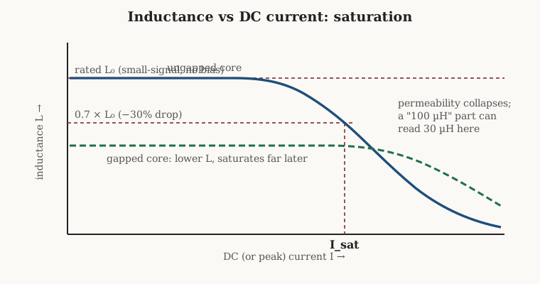
This is the origin of a fact that startles newcomers: an inductor sold as “100 µH” can measure 30 µH — or less — when it is actually carrying its rated current, because at that current the core is well into saturation. Manufacturers cope by defining a saturation current rating, I_sat, as the DC current at which the inductance has dropped by some stated fraction from its zero-current value. Coilcraft, for example, typically publishes the current for a 10 %, 20 %, and 30 % drop; other makers pick a single threshold. There is nothing fundamental about 30 % — it is a convention — so two parts are only comparable at the same drop percentage, and a designer must read which threshold a datasheet used before trusting the number. In a switching supply, saturation is not gentle: as the inductor loses inductance the current ramp steepens, which drives the core further into saturation, and the current can run away to destruction within a single switching cycle. Saturation is a hard wall to design behind, not a soft limit to nibble at.

Temperature makes it worse, because B_sat falls as the core warms. A manganese-zinc power ferrite might hold roughly 0.4–0.5 T at room temperature but only around 0.3 T at 100 °C, so a hot inductor saturates at a lower current than the same part measured cold — precisely the wrong direction, since the part is usually hot because it is working hard. Different core families set very different ceilings: ferrites saturate low, around 0.3–0.5 T; powdered-iron and other distributed-gap powder cores run higher, roughly 1.0–1.5 T, and saturate gracefully; silicon-steel laminations reach 1.5–2.0 T. The core volume tabulates them.

2.9.1 The air gap: trading inductance for headroom

The classic fix for saturation is to cut a small air gap into the magnetic path — a physical slot in a ferrite E-core, or the distributed micro-gaps built into a powdered core. It seems perverse to deliberately break the magnetic circuit, but the effect is exactly what a saturation-limited design wants.

The gap adds a large, linear reluctance in series with the low-reluctance iron. Because the gap dominates, the effective permeability of the whole magnetic circuit drops — so the inductance for a given number of turns falls, and it becomes far less sensitive to the exact permeability of the ferrite. In exchange, the same ampere-turns now produce far less flux density in the core, so it takes much more current to reach B_sat: the saturation curve flattens out and slides to the right, exactly the gapped curve in Figure 5. Seen from the energy side, a gapped inductor stores most of its energy in the gap rather than in the iron, and air cannot saturate — which is why any inductor meant to store energy against a DC bias, as in a buck or boost converter, is gapped or built on a distributed-gap powder core. The price is paid in turns: to recover the lost inductance the winder adds turns, which adds DCR and winding capacitance, closing the loop back to the earlier parasitics. The core volume covers gap calculation and the A_L factor; here the gap is simply the standard lever for buying saturation headroom.

2.10 Temperature: two different current limits

The discussion of saturation and of copper loss exposes something a beginner rarely expects — an inductor has two independent current ratings, set by two unrelated failure modes, and the lower of the two governs.

The first is I_sat, the magnetic limit just discussed: exceed it and the inductance collapses. The second is I_rms, a thermal limit: it is the RMS current that raises the part’s temperature by a specified amount above ambient through I²·R heating, independent of whether the core is anywhere near saturation. Manufacturers pick a temperature-rise budget for the rating — Coilcraft, for instance, typically uses a 15 °C rise for small chip inductors and 40 °C for power inductors — measured in still air with the part self-heating. Exceed I_rms and nothing dramatic happens to the inductance; the part simply overheats, cooks its own insulation, and eventually fails.

Crucially the two ratings are set by different physics and can fall either side of one another. For a small ferrite inductor the core often saturates before it gets hot, so I_sat is the lower number and governs. For a robust powder-core choke with a high saturation ceiling, the copper reaches its thermal limit first, so I_rms governs. A datasheet worth reading gives both, and a design must clear both — a part that comfortably passes the thermal rating is still ruined if a fault transient pushes it past saturation. Temperature also shifts the inductance itself: the core’s permeability drifts with temperature, so the nominal L wanders by a few percent to a few tens of percent over the operating range depending on the material, and the copper’s DCR climbs by roughly 0.39 % per degree as already noted. The stable-across-temperature inductor and the high-density inductor are, as usual, different parts.

2.11 Reading an inductor datasheet

Every parasitic in this volume appears, named, in the specification table of a real part, and reading one is a matter of knowing which limit each number guards.

Take a representative shielded power inductor of, say, 10 µH. Its inductance is quoted with a tolerance (±20 % is common) and — importantly — at a stated small-signal test frequency and zero DC bias, which is the headline value, not the value it will show in circuit. Its DCR might read a few tens of milliohms; multiply the square of the working current by it to find the copper loss and hence much of the heating. Its I_sat is given at a stated inductance-drop percentage — check whether it is 10, 20, or 30 % before comparing parts — and is the current below which the inductance stays honest. Its I_rms is given with a stated temperature rise (15 °C or 40 °C, typically) and is the current below which the part stays cool; the working current must sit under both. Its SRF, perhaps a few tens of megahertz for a part this size, marks where it stops being an inductor, and the operating and switching frequencies must live well below it. An RF-oriented part adds a Q figure quoted at a specific frequency, the number that decides how sharp a tuned circuit it can make.

Line those six parameters up against the equivalent circuit of Figure 1 and the datasheet stops being a list and becomes a portrait: L is the ideal element, DCR is the series resistor, SRF is L resonating with C_w, Q folds DCR and R_core together, I_sat is the flux ceiling, and I_rms is the thermal one. The ideal inductor of the foundational volume is where design starts; this collection of losses, limits, and hidden reactances is the component that actually gets soldered down, and every later volume — the cores that set saturation and loss, the wire that sets DCR and skin effect, the winding craft that sets C_w and SRF, and the measurement bench that pins all of it down — is a deeper look at one corner of this same picture.