Designing and Calculating Inductors

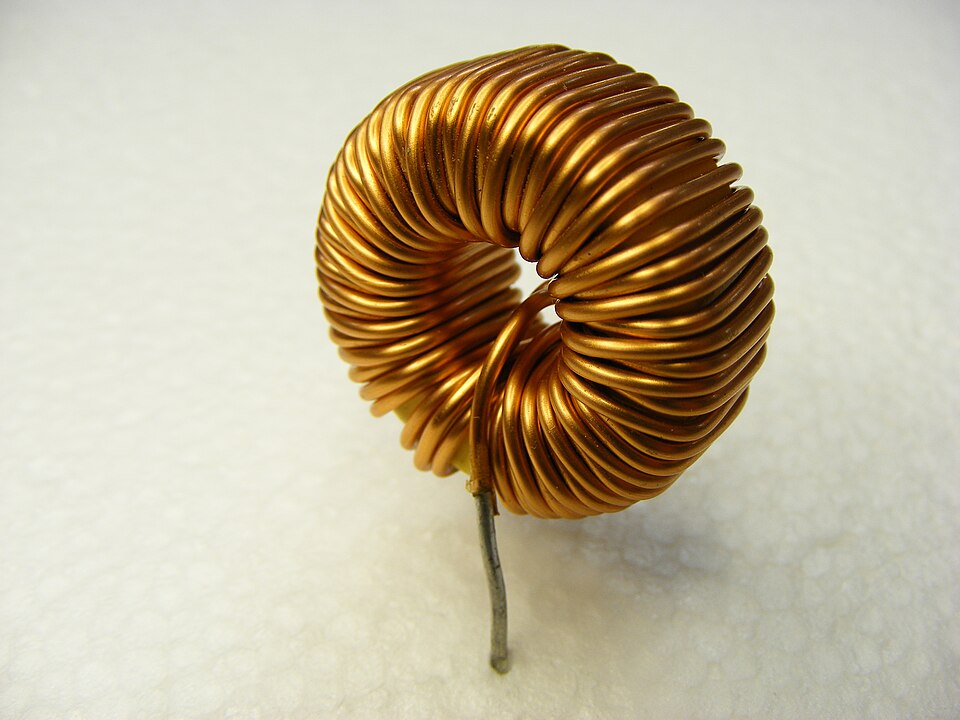
9.1 From a number on a schematic to turns on a former

Every volume so far has treated inductance as something a coil simply has — a property to be measured, drawn as a squiggle, and reasoned about. This volume runs the arrow the other way. It starts with a number the circuit demands — “give me 2.5 µH here,” or “100 µH that holds up at three amps” — and works backward to the physical object: which core, how many turns, what wire, wound how long. This is the design problem, and it is the moment the abstraction becomes brass, ferrite, and enamelled copper.

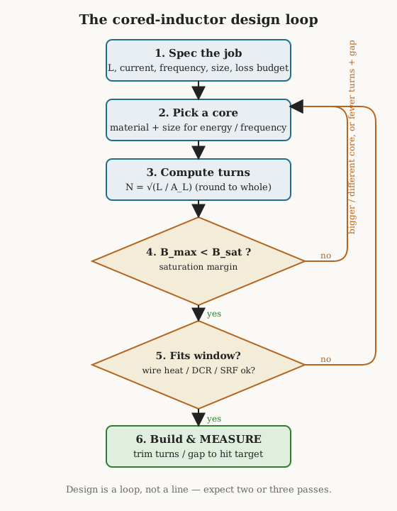
The good news for the newcomer is that the arithmetic is mostly algebra a schoolchild could do. The good news for the engineer is that the arithmetic is never the hard part. The hard part is that a coil must satisfy several constraints at once — the right inductance, but also small enough to fit, cool enough not to cook, linear enough not to saturate, and resonance-free across its operating band — and improving one usually worsens another. Design is therefore not a formula but a loop: propose a coil, check every constraint, and go around again when one fails. Nobody nails a power inductor on the first pass. The professionals simply lose fewer laps.

9.1.1 What the spec actually contains

Before a single turn is counted, five quantities have to be pinned down, because they decide everything downstream:

• Inductance, L — the headline value, in henries (usually µH or mH). It sets the turns.
• Current — both the RMS current (which heats the wire) and the peak current (which sets the flux and therefore whether the core saturates). These are different numbers and both matter; conflating them is the classic beginner’s error.
• Frequency — the operating frequency, and for switching converters the ripple frequency, which drives core loss and decides the core material.
• Size and shape — the box the coil must fit in, and often the mounting style.
• The loss / temperature budget — how much heat the thing is allowed to make, set by efficiency targets and by how hot the surroundings already are.

Two of these — the inductance and the core material and geometry — come straight out of earlier volumes. The core-materials volume is where permeability, saturation flux density, the A_L index, and gapping were defined; this volume simply uses those numbers. The wire volume supplies gauge, resistance-per-metre, and the fill-factor reality that decides whether a winding physically fits. What follows assumes those inputs and concentrates on the calculation and the checks.

9.2 Air-core design: Wheeler’s solenoid

When there is no core — just wire wound on a plastic, ceramic, or air former — the inductance comes entirely from geometry. There is no permeability to lean on, no saturation to fear, and no core loss; an air-core coil is beautifully linear and stable, which is exactly why RF designers reach for it in tuned circuits and why it reappears wherever a few hundred nanohenries to a few tens of microhenries are needed at high frequency. The price is size: with no core to concentrate the flux, air-core coils are physically large for their inductance, and above a handful of microhenries they become impractically bulky.

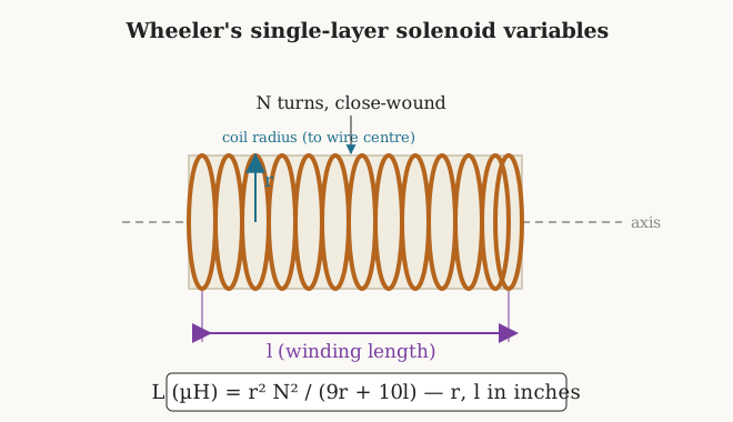
The workhorse formula for the single-layer solenoid — a single helical layer of turns on a cylindrical former — is Wheeler’s equation, published by Harold Wheeler in 1928 and reprinted in every serious reference from Terman to the ARRL Handbook. In its classic English-unit form:

L (µH) = r² N² / (9r + 10l)

where r is the coil radius in inches (to the centre of the wire), l is the winding length in inches, and N is the number of turns. It is an empirical approximation, not an exact result — Wheeler fitted it to the true field solution — but for ordinary coil proportions it lands within about 1%, which is far tighter than the tolerance of the wire, the former, or the winder’s hands. The catch is its validity range: the approximation holds when the coil is not too short, roughly l ≳ 0.4r, and is at its ~1% best when l ≳ 0.8r. A squat pancake of a coil (length much less than its radius) needs a different formula; a normal solenoid is squarely in Wheeler’s territory.

9.2.1 Worked example: a 2.2 µH RF coil

Suppose the circuit wants 2.2 µH for a high-frequency tuned stage, and the bench has a former of 0.5 inch diameter (so radius r = 0.25 in) and a spool of 24 AWG enamelled wire. From the wire volume, 24 AWG over its enamel is about 0.022 in in diameter, so a close-wound turn advances the winding by roughly that much: the length is l ≈ 0.022·N inches. There are two unknowns, N and l, but they are tied together by the close-wind pitch, so the problem collapses to one equation.

Substitute l = 0.022N into Wheeler’s formula and set L = 2.2:

2.2 = (0.25)² N² / (9·0.25 + 10·0.022N)
2.2 = 0.0625 N² / (2.25 + 0.22N)

Multiply out:

2.2 · (2.25 + 0.22N) = 0.0625 N²
4.95 + 0.484N = 0.0625 N²
0.0625 N² − 0.484N − 4.95 = 0

A quadratic in N. Solving (multiplying through by 16 to tidy it):

N² − 7.744N − 79.2 = 0
N = [7.744 + √(7.744² + 4·79.2)] / 2
N = [7.744 + √376.8] / 2 = [7.744 + 19.41] / 2 ≈ 13.6 turns

Turns come in whole numbers, so the real choice is 13 or 14. Checking each back through Wheeler:

• 14 turns: l = 14·0.022 = 0.308 in; L = 0.0625·196 / (2.25 + 3.08) = 12.25 / 5.33 = 2.30 µH
• 13 turns: l = 13·0.022 = 0.286 in; L = 0.0625·169 / (2.25 + 2.86) = 10.56 / 5.11 = 2.07 µH

Fourteen turns overshoots slightly, thirteen undershoots. This is the everyday reality of coil design: the answer is rarely an integer, and the builder either accepts the nearest whole turn or, on an air-core coil, stretches or squeezes the winding to trim the value — spreading 14 turns very slightly lengthens l and pulls the 2.30 µH back down toward 2.2. That live adjustability is one of the quiet pleasures of air-core work, and the measurement volume shows how to dial it in on an LCR meter.

One design choice Wheeler does not decide is spacing. Close-winding packs the most turns into the least length and is simplest, but at high frequency the proximity effect between snug turns drags the Q down. Where Q is precious, RF coils are deliberately space-wound — turns separated by roughly a wire diameter — which raises Q at the cost of a longer coil and slightly fewer turns for the same length. Spacing also lifts the self-resonant frequency, since it thins the turn-to-turn capacitance. It is a lever worth remembering: the same 2.2 µH can be a short close-wound coil or a longer airy one, and the choice is made on Q and SRF, not on inductance.

Check the geometry against Wheeler’s validity rule: with 14 turns, l/r = 0.308 / 0.25 = 1.23, comfortably past the 0.8 threshold, so the ~1% accuracy holds. And a sanity check on self-resonant frequency: a single-layer solenoid this size has a self-capacitance of well under a picofarad (Medhurst’s data for these proportions puts it near 0.7 pF). With L = 2.3 µH and C ≈ 0.7 pF, the SRF is roughly

f_SRF = 1 / (2π√(LC)) = 1 / (2π√(2.3e-6 · 0.7e-12)) ≈ 125 MHz

— comfortably above any HF operating frequency, so the coil behaves as an inductor, not as a stray resonator, where it will be used. (Medhurst’s self-capacitance figures are approximations; the real number is confirmed on the bench, not trusted from a table.) The coil fits, is stable, dissipates essentially nothing, and needs no core. For 2 µH that is a fine trade. For 200 µH it would be the size of a soup can, which is why the next section reaches for a core.

9.2.2 Multilayer and why it is fuzzier

Stack the winding into several layers and the inductance climbs fast — each layer sees the flux of all the others — but the tidy single-variable geometry is gone. The standard multilayer estimate is Wheeler’s second formula, which adds the winding depth (the radial build of the coil) as a third dimension alongside radius and length. It is inherently less accurate than the single-layer form, typically a few percent, because the exact answer depends on how the turns actually nest layer to layer — and real windings are never the ideal brick of copper the formula imagines. Multilayer air-core coils (and their scatter-wound, universal, and honeycomb cousins from the geometries volume) are therefore designed with more slack and always measured afterward. The lesson generalises: the more turns and the messier the winding, the more the calculation is a starting point rather than an answer.

9.3 Cored design by the A_L value

Add a magnetic core and the game changes entirely. A high-permeability core multiplies the inductance of a given winding by a large factor, so the same 100 µH that needed a soup can of air-core wire now needs a dozen turns on a thumbnail-sized toroid. The core also concentrates and confines the flux — a toroid is nearly self-shielding — which is why cored inductors dominate everywhere except the highest-Q RF work.

The everyday design method for a core is the A_L value, and it is refreshingly simple. The manufacturer has already done the magnetics: for a given core, A_L is the inductance per turn squared — a single number that folds in the core’s permeability, its cross-section, and its magnetic path length. Because inductance scales with the square of the turns (double the turns, quadruple the flux linkage), the whole relationship is just:

L = A_L · N² and therefore N = √(L / A_L)

The only trap is units, because three conventions are in common use and mixing them produces answers wrong by factors of 100 or 10,000:

• nH/N² (Micrometals, most datasheets): L in nH, so L = A_L · N², N = √(L_nH / A_L).
• µH per 100 turns (Amidon iron-powder “T” cores): L = A_L · (N/100)², so N = 100·√(L_µH / A_L).
• mH per 1000 turns (Amidon ferrite “FT” cores): L = A_L · (N/1000)², so N = 1000·√(L_mH / A_L).

They describe the same physics; a core listed as 4 nH/N² is identically 40 µH/100 turns. The disciplined habit is to write the units next to every A_L and cancel them explicitly, exactly as one would with any other engineering quantity.

9.3.1 Worked example: 2.5 µH on an iron-powder toroid

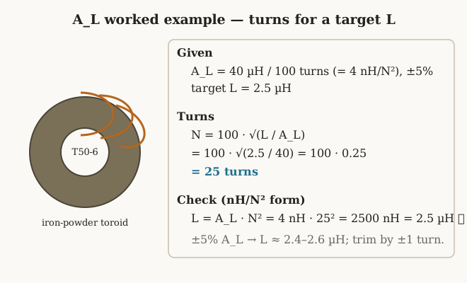
Take the same 2.5 µH but built as a small RF choke on a well-known iron-powder core, the Amidon T50-6 (mix 6, the yellow carbonyl-iron material used from a few MHz to about 40 MHz). Its published index is A_L = 40 µH per 100 turns, equivalently 4 nH/N², with a ±5% tolerance. (A quick physics check confirms the catalogue figure: with mix-6 permeability µ ≈ 8.5, an effective area A_e ≈ 12 mm², and a mean path l_e ≈ 32 mm, µ₀·µ·A_e/l_e works out to about 4 nH/turn² — the manufacturer’s number, not an invented one.)

Turns for 2.5 µH:

N = 100 · √(L / A_L) = 100 · √(2.5 / 40) = 100 · √0.0625 = 100 · 0.25 = 25 turns

Cross-check in the nH/N² convention: L = 4 nH · 25² = 4 · 625 = 2500 nH = 2.5 µH. ✓ The two unit systems agree, which is the whole reason to carry the units through.

Now walk the checks, because the turns count is only the first of them:

• Does it fit the window? The T50-6 has an inner diameter of 7.7 mm, so the inner circumference is π·7.7 ≈ 24.2 mm. Twenty-five turns of 26 AWG wire (about 0.45 mm over the enamel) occupy 25·0.45 ≈ 11.3 mm of that inner ring — under half — so the winding fits comfortably in a single layer with room to spare. (Turns crowd toward the inner hole of a toroid, so the inner circumference, not the outer, is the binding dimension. When a single layer will not fit, the winder either drops to finer wire or moves up a core size — that is the “no” branch of the design loop.)
• DCR and heating. The mean length of a turn on a T50-6 is about 15 mm, so 25 turns is roughly 0.375 m of 26 AWG wire. At ~0.13 Ω/m that is about 50 mΩ of DC resistance — negligible for a small-signal RF choke, and a temperature rise of nothing worth calculating.
• Saturation. This is where iron powder behaves differently from ferrite, and the distinction matters. Iron-powder cores have a distributed air gap — microscopic iron particles insulated from one another — so they do not have a sharp saturation knee. Instead the permeability rolls off gradually with flux; full saturation for carbonyl iron is up around 10,000 gauss (1 T), but the material is soft long before that. In practice, iron-powder RF and power designs are almost always limited by temperature rise from core loss, not by saturation, so for a small-signal choke like this one the saturation check is a formality. When it does matter (an iron-powder power choke carrying real DC), the check is the same flux calculation used for ferrite below.

Finally, note the A_L tolerance. At ±5%, the 2.5 µH target is really 2.4–2.6 µH before the coil is even wound; iron-powder A_L also drifts a little with temperature (mix 6 has a temperature coefficient around 35 ppm/°C). For a tuned circuit that must land on a precise value, the coil is wound a touch high and tapped or unwound turn-by-turn while watching the meter — again, the design gives the turns, the bench gives the value.

9.4 Energy-storage inductors: designing for power

RF chokes and tuned coils carry little energy; power inductors are built to store it. The output inductor of a switching converter, the choke in a boost or flyback — these spend their lives shuttling energy between magnetic field and circuit on every switching cycle, and the governing quantity is not inductance alone but the energy the coil can hold without saturating:

W = ½ L I²

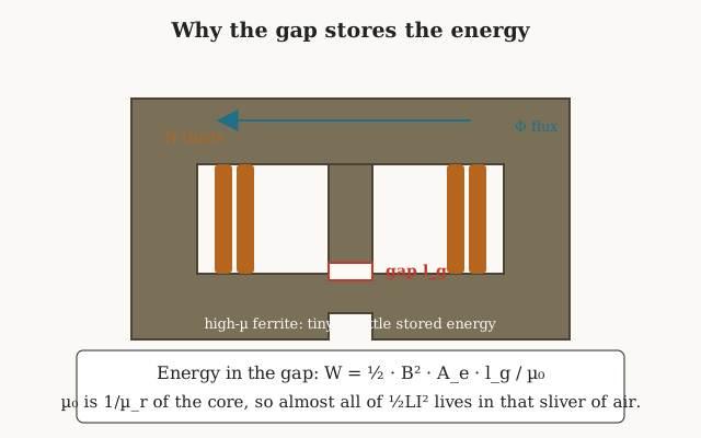
Here is the fact that shapes every power-inductor design: a high-permeability core stores almost no energy — the energy lives in the air gap. Energy density in a magnetic material goes as B²/2µ, and because a ferrite’s µ is thousands of times that of air, a given flux density stores thousands of times less energy in the ferrite than in an equal volume of gap. A solid, ungapped ferrite core saturates almost immediately under DC bias precisely because it has nowhere to put the energy. Cut a gap — or use a powder core, whose distributed particle-to-particle gaps do the same job throughout the volume — and the coil suddenly holds real energy, because that energy is now stored in the low-permeability gap where the flux density can be high without the material minding.

9.4.1 The two currents, and the two ways to fail

Before any turns are computed, a power inductor forces a distinction the small-signal world lets one ignore: there are two currents and they break the coil in two different ways. The peak current — DC load plus half the peak-to-peak ripple — sets the peak flux density, and if that flux reaches B_sat the inductance collapses, the current runs away in an instant, and the converter’s switch usually dies with it. Saturation is a fast, catastrophic failure driven by the peak. The RMS current, by contrast, sets the I²R heating in the copper and the AC loss in the core, and those raise the temperature slowly; too much and the winding cooks, the insulation degrades, and — because B_sat itself sinks with temperature — the saturation margin quietly erodes until the coil that was fine cold saturates hot. Overheating is a slow failure driven by the RMS. A finished design has to clear both hurdles at once: B_pk(I_pk) < B_sat(hot) and temperature rise from I²_rms·R plus core loss within budget. They pull in opposite directions — surviving the peak wants a bigger gap and more turns, surviving the RMS wants fatter, lower-resistance wire — and the core has to have room for both. That tension is the whole reason a power inductor is bigger than its inductance alone would suggest.

9.4.2 Sizing the core before counting turns

How does one pick the core in the first place, before N is known? The professional shortcut is the energy-storage (or area-product) view. A core can hold only so much energy before it saturates, and that ceiling scales with the product of its magnetic cross-section A_e and its window area W_a — the area product, A_p = A_e·W_a — because A_e limits the flux and W_a limits the copper. Design references tabulate an A_p (or a related “energy-handling”) figure for every stock core, so the flow is: compute the stored energy ½LI²_pk, look up the smallest core whose area product covers it with margin, and then run the turns-and-gap arithmetic above to confirm. It turns core selection from guesswork into a lookup, and it is why manufacturers publish selector charts keyed to inductance-times-current-squared. The worked example below skipped straight to a plausible 80 mm² core; in practice that first choice comes from an A_p chart or a manufacturer’s online selector, and the checks either bless it or send the design one core size up.

The gapped-core relationships follow from the magnetic circuit. With a gap long enough to dominate the reluctance (true for any useful ferrite gap), the inductance is set by the gap almost alone:

L ≈ µ₀ N² A_e / l_g

and the peak flux density in the core — the number that must stay under B_sat — is

B_pk = L · I_pk / (N · A_e) = µ₀ N I_pk / l_g

where A_e is the core’s effective cross-section, l_g the total gap length, and I_pk the peak current. These two equations, plus the energy relation, are the entire toolkit.

9.4.3 Worked example: a 100 µH buck-converter inductor

Design the output choke for a buck converter: target L = 100 µH, peak current I_pk = 3 A, RMS current about 2.5 A. The peak energy the coil must hold is

W = ½ L I_pk² = ½ · 100e-6 · 3² = ½ · 100e-6 · 9 = 450 µJ

That energy figure is what sizes the core — big enough to hold 450 µJ in its gap without the flux running away. Pick a gapped MnZn power-ferrite core (an N87-class material, say) with an effective area A_e ≈ 80 mm² = 80×10⁻⁶ m², a common size for this power level.

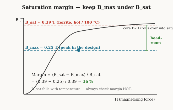
Step 1 — choose the peak flux, then get the turns. This is the design’s pivot: rather than guess turns and hope, decide how much flux density to allow and let it fix N. MnZn power ferrite saturates around B_sat ≈ 0.39 T when hot (100 °C) — and hot is the condition that counts, because B_sat falls with temperature. Target a peak of B_pk = 0.25 T, leaving healthy margin. Rearranging the flux equation for N:

N = L · I_pk / (B_pk · A_e)
N = (100e-6 · 3) / (0.25 · 80e-6)
N = 3e-4 / 2e-5 = 15 turns

Step 2 — set the gap for the inductance. With N fixed at 15, solve L ≈ µ₀N²A_e/l_g for the gap:

l_g = µ₀ N² A_e / L
l_g = (4π×10⁻⁷ · 15² · 80e-6) / 100e-6
l_g = (1.257e-6 · 225 · 80e-6) / 100e-6
l_g ≈ 2.26e-4 m = 0.226 mm

A gap of about 0.23 mm — a couple of business-card thicknesses of shim, or a ground centre-leg — gives 100 µH at 15 turns. (In an E-core one either grinds the centre leg by this amount or splits it as ~0.11 mm shims under each outer leg.)

Step 3 — confirm the saturation margin, hot. Recompute B_pk with the final numbers to be sure nothing drifted:

B_pk = µ₀ N I_pk / l_g = (1.257e-6 · 15 · 3) / 2.26e-4 ≈ 0.25 T

Against B_sat ≈ 0.39 T at 100 °C, the margin is (0.39 − 0.25)/0.39 ≈ 36% — solid headroom for load transients and temperature. If a transient could push I_pk higher, the fix is more turns and a longer gap (lower B_pk), at the cost of more copper.

Step 4 — the beautiful check. Compute the energy stored in the gap and confirm it equals ½LI²:

W_gap = ½ · B_pk² · A_e · l_g / µ₀
W_gap = ½ · 0.25² · 80e-6 · 2.26e-4 / 1.257e-6
W_gap = ½ · 0.0625 · 80e-6 · 2.26e-4 / 1.257e-6 ≈ 4.5e-4 J = 450 µJ

Exactly the ½LI² from the start. The energy really is in the gap, and the arithmetic closes on itself — a satisfying confirmation that the model is self-consistent.

Step 5 — wire, window, heating. The winding carries 2.5 A RMS. At a conservative current density of ~4 A/mm² that wants about 0.6 mm² of copper — roughly 19 AWG (0.65 mm²). Fifteen turns of 19 AWG is a small winding that fits an E25-class bobbin window easily. DCR: at a ~50 mm mean turn, the wire length is 15·0.05 = 0.75 m; at ~26 mΩ/m for 19 AWG that is about 20 mΩ. Copper loss is then I²R = 2.5² · 0.02 ≈ 0.13 W — modest, and added to the core’s AC loss it gives a temperature rise a designer would happily accept. The coil passes every check on the first honest pass; real designs often do not, and go back to Step 1 with a bigger core or a different B_pk target.

The powder-core alternative to all of this is to skip the discrete gap and use a distributed-gap material — sendust (Kool Mµ), MPP, or high-flux powder — whose gap is spread through the whole volume. The design flow is identical, but instead of choosing a gap length one chooses a permeability mix, then reads a percent-of-rated- inductance versus DC-bias curve from the datasheet to confirm the inductance does not sag too far under the DC current. Powder cores trade a little more core loss for a gentler saturation and no fringing-field losses around a discrete gap — which is why they dominate modern SMPS output chokes.

9.5 The checks every design must pass

The worked examples exercised the checks in passing; it is worth stating them as a set, because a coil that hits its inductance and fails any one of these is not a finished design. Each of them is a design constraint version of a parasitic the real-inductor volume introduced — saturation, self-resonance, Q, and DCR are the non-ideal behaviours of an actual coil, and here they simply become the pass/fail lines a new design must clear.

• Saturation margin. Peak flux density, computed from peak current (DC bias plus AC ripple), must sit safely under B_sat — and B_sat must be the hot value, because it falls with temperature and a coil that is fine on the bench can saturate at full load. Comfortable margins are 20–40%. Iron-powder and other distributed-gap cores substitute a permeability-versus-bias curve for a hard B_sat, but the intent is the same: keep the inductance from collapsing under current.

• Self-resonant frequency. Every winding has self-capacitance, and above the SRF the coil is a capacitor, not an inductor. The SRF must sit comfortably above the highest frequency of interest — a factor of several is the usual comfort zone. This bites hardest on many-turn RF chokes, where the geometries volume’s universal and honeycomb windings exist precisely to push self-capacitance down and SRF up.

• Q and loss at frequency. For a tuned or resonant application the coil’s Q — set by DCR at low frequency, and by skin effect, proximity effect, and core loss as frequency climbs — must be high enough. This is where wire choice (and Litz, from the wire volume) and core material earn their keep.

• DCR and temperature rise. The RMS current through the DC resistance makes I²R heat; core loss adds more. Together they set the temperature rise, which must stay within the wire’s insulation class and the enclosure’s budget. A coil that meets its inductance but runs at 130 °C in a 105 °C-rated winding has failed.

• Window fit and fill factor. The computed turns of the chosen wire have to physically go into the winding window. Round wire cannot fill a window completely — a copper fill factor of 0.4–0.6 is typical after insulation, layer clearances, and the geometry of round turns in a rectangular window — so a winding that looks like it fits on paper may not fit in fact. This is a hard, unforgiving constraint, and it is the one most often discovered too late.

9.6 Practical realities and a design recipe

Two honest admissions run through everything above. First, the inputs are tolerant. A_L is a specification with a spread, not a constant: ±5% is typical for iron powder, ±3% down to ±25% for various ferrites depending on grade and whether the core is gapped, and an ungapped high-permeability ferrite can vary its A_L by tens of percent because it directly inherits the material’s loosely-controlled permeability. Gapping a core, ironically, tightens its A_L tolerance — once the gap dominates the reluctance, the inductance depends mostly on gap geometry and hardly at all on the core’s exact µ, which is one more reason power designs gap. On top of the manufacturing spread, permeability drifts with temperature (iron-powder mixes carry a stated ppm/°C coefficient; ferrite µ can swing widely and non-monotonically across its operating range and peaks near the Curie temperature just before it falls off a cliff), the wire diameter varies within its own gauge tolerance, and real windings never nest into the perfect brick the formulas assume. Stack these up and the calculated inductance is a best-estimate with a real error bar around it — a design that only just meets a tight tolerance on paper will miss it in copper often enough to matter.

Second, and following directly: the real value is the measured value. Serious coil work is build-and-measure. The calculation gets the turns close enough that the first prototype is in the right neighbourhood; the LCR meter — the subject of the measurement volume — gets it exact. When the measurement disagrees with the target, the trims are familiar: add or remove turns (each turn moves L by roughly 2N/N² ≈ 2/N of its value near the target); spread or compress an air-core winding; widen or shim a ferrite gap; or bring out a tap so the value can be selected after the fact.

The whole method, distilled to something the reader can actually follow at the bench:

1. Write the spec — L, peak and RMS current, frequency, size, temperature budget.
2. Choose the core — material for the frequency and loss, size for the energy (½LI²) and the space. Air core for small, high-Q RF; iron powder or ferrite for the rest; gapped ferrite or distributed-gap powder for energy storage.
3. Compute the turns — Wheeler for a single-layer air coil; N = √(L/A_L) for a core, with the units written out.
4. Check saturation — B_pk = L·I_pk/(N·A_e) against B_sat hot, with margin.
5. Check the winding — does the wire fit the window; is the DCR and its I²R heat acceptable; is the SRF well above the operating band; is Q high enough?
6. Iterate — any failed check sends the design back to a bigger core, different turns, or a different gap. Expect two or three laps.
7. Build and measure — wind it, put it on the meter, and trim turns or gap until it is right.

The next volumes take this recipe into the shop. The winding-technique volume covers actually laying down the computed turns — tension, layering, and the toroid-by-hand method that turns “25 turns of 26 AWG” into a real coil — and the measurement volume covers putting the finished coil on an LCR meter to confirm that the number on the schematic finally, honestly, matches the object on the bench.