The Real Resistor: Tolerance, Tempco, Noise, and Parasitics

3.1 The gap between the symbol and the part

On a schematic a resistor is a single zig-zag or a plain rectangle and a single number: 10 kΩ. That symbol promises a great deal. It promises a resistance that is exactly ten thousand ohms; that stays ten thousand ohms whether the room is freezing or the part is running hot; that is ten thousand ohms whether one volt or one hundred volts sits across it; that behaves the same at DC as it does at a hundred megahertz; and that adds nothing of its own to the signals passing through it — no drift, no distortion, no hiss. That is the ideal resistor: a pure, constant, frequency-independent, noiseless resistance.

No real resistor keeps all of those promises, and a surprising number of bench problems come down to discovering which promise a particular part has quietly broken. This volume is about the difference between the symbol and the object — the systematic ways every physical resistor departs from its ideal, and how much each departure actually costs the designer.

It is the direct sibling of two volumes elsewhere in this passive-components program. The Capacitors dive has a volume on the real capacitor — the one with equivalent series resistance (ESR), equivalent series inductance (ESL), dielectric loss (dissipation factor), and a self-resonant frequency where it stops being a capacitor at all. The Coils dive has the matching volume on the real inductor — the one with winding resistance (DCR), a finite quality factor Q, inter-winding capacitance, and its own self-resonance. Each of those volumes takes an idealized textbook element and asks what the physical part really does. This volume does exactly the same job for the resistor, and it turns out the resistor, humble as it looks, has just as rich a set of non-idealities as its reactive cousins. The reader who has absorbed ESR and SRF will find the vocabulary here familiar; a resistor is simply a component whose intended behaviour is the pure real part, with a set of parasitic reactances and error terms wrapped around it.

Here is the roadmap of deviations, in the order they are treated below. First, tolerance: the resistance is not the marked value but somewhere in a band around it. Second, temperature coefficient (tempco, or TCR): the resistance changes as the part warms and cools. Third, the voltage coefficient (VCR): the resistance changes slightly with the voltage across it. Fourth, the equivalent circuit and the frequency response that follows from it: the real part is not a pure resistance but a resistance dressed in a little series inductance and a little shunt capacitance, so its impedance walks away from the nominal value at high frequency. Fifth, noise, in two distinct flavours — the unavoidable thermal floor present in any resistance, and the excess “current” noise that only some construction types add on top. Sixth, stability and drift over the life of the part. And last, a brief word on power derating, before a closing table that scores each common resistor type across all of these axes so the reader can see the whole trade-space at a glance.

3.2 Tolerance: why a “1 kΩ” is never exactly 1 kΩ

The most familiar deviation is the one printed right on the part. A resistor marked 1 kΩ with a 5% tolerance is not promised to be 1000 Ω; it is promised only to fall somewhere between 950 Ω and 1050 Ω. Tolerance is the manufacturer’s guarantee about the spread of production, not a statement about any individual piece. Buy a thousand of them, measure each on a good meter, and the values scatter across that hundred-ohm-wide band.

For the layman the mental model is a factory that cannot make anything perfectly. The resistive element — a film, a rod, a length of wire — is deposited or wound to a target, but every physical process has variation: film thickness wanders, trimming stops a hair early or late, materials differ batch to batch. The tolerance band is the honest admission of how tightly the process can be held. A tighter band costs more because it demands better process control or a post-production sort.

For the engineer the important subtleties are three. The first is that tolerance is tied to the E-series value ladder — the standardized set of preferred values (E6, E12, E24, E96, and so on) that the coming Volume 6 treats in full. The spacing of those values is not arbitrary; it is chosen so that the tolerance bands tile the number line with no gaps. The E24 series (used for 5% parts) steps by roughly 10% from one value to the next — 910 Ω, 1.0 kΩ, 1.1 kΩ — precisely so that a ±5% band around each value just meets the band around its neighbour. Every possible resistance is covered by exactly one preferred value’s tolerance band; the ladder is engineered around the spread. Tighter parts need a finer ladder: the E96 series (for 1% parts) has ninety-six steps per decade because a ±1% band is only a fifth as wide and needs correspondingly closer rungs to tile the line. Tolerance and the value ladder are two views of the same design.

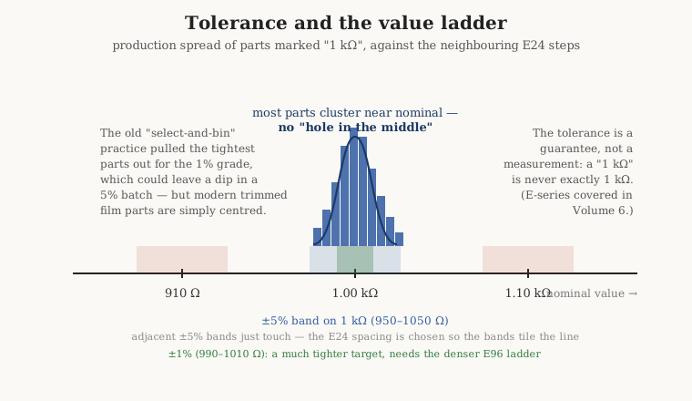
The second subtlety is historical and it concerns the shape of that distribution. In the era of loosely-controlled carbon parts, manufacturers practised select-and-bin: they made resistors to a wide spread and then sorted them by measurement. The pieces that came out closest to nominal were pulled and marked with the tight tolerance and sold at a premium; what remained — the parts that had missed the centre — were marked to the looser grade. This gave rise to a persistent piece of workshop folklore: that a batch of 5% resistors has a “hole in the middle,” a dip in the distribution right at the nominal value, because all the good ones were skimmed off for the 1% bin. There is a grain of truth to it for old select-and-binned stock. But it is a myth for essentially everything a designer buys today. Modern film resistors are trimmed — a laser or an abrasive jet cuts the element while the value is measured live, and the cut stops when the target is hit — so each part is actively steered toward nominal. The resulting distribution is roughly Gaussian and densest at the centre, the opposite of a hole. A modern 1% metal-film part is not a lucky survivor from a 5% pool; it was made to be 1%.

The third subtlety is the design discipline that follows from all this: never assume the nominal. A divider, a gain-setting pair, a current-sense value — each must be analysed for the worst-case corners of its tolerance band, and often for the combination of several parts drifting to their opposite extremes at once. A designer who wants a ratio held to 0.1% cannot build it from 1% parts and hope; either tighter parts are specified, or — as the tempco discussion below shows — a matched network is used so that the errors cancel rather than add.

3.3 Temperature coefficient: the value that moves with the weather

A resistor’s value changes with temperature. The temperature coefficient of resistance, TCR or tempco, quantifies how much, and it is quoted in parts per million per degree Celsius, written ppm/°C. One part per million is 0.0001%, so a tempco of 100 ppm/°C means the resistance shifts by 0.01% for every degree of temperature change.

The worked example makes it concrete. Take a 10 kΩ resistor with a tempco of 100 ppm/°C — an unremarkable metal-film figure — and warm it by 50 °C, which is easily done by a hot summer enclosure or by the part’s own dissipation. The change is

ΔR = R × TCR × ΔT = 10 000 Ω × 100×10⁻⁶ /°C × 50 °C = +50 Ω,

or +0.5%. That is worth pausing on: a 0.5% shift from temperature alone is five times larger than the initial tolerance of a 0.1% part. A designer who pays for tight tolerance and ignores tempco has bought precision that the first warm afternoon erases.

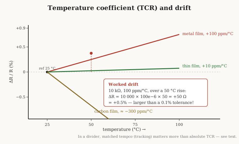
The sign and shape of the tempco depend on the resistive material, and the spread across types is wide. Bulk metal foil parts are the aristocracy at under 1–2 ppm/°C; precision wirewound made from Evanohm and similar alloys reaches 1–3 ppm/°C. Thin-film chip resistors sit at 5–25 ppm/°C, good enough for most instrumentation. Ordinary metal-film axials run 50–100 ppm/°C. Thick-film chips — the workhorse of every mass-produced board — are typically ±100 to ±200 ppm/°C, and often quoted at ±200. Carbon-film parts have a negative tempco, roughly −200 to −500 ppm/°C, so they fall in value as they warm. Carbon composition is the wild one: its tempco is large, can reach hundreds of ppm and beyond (figures toward +1200 ppm/°C appear), and it is non-monotonic — the value dips and then rises across the temperature range rather than tracking a straight line, which makes it nearly impossible to compensate. These figures are the ones cited by the major makers — Vishay, Yageo, KOA Speer, Susumu — and they are the first thing a precision designer looks up.

Now comes the single most useful idea in this section, and it separates the engineer from the novice. In a great many circuits the resistor does not act alone; it acts in a ratio. A voltage divider, a bridge, a gain-setting pair around an op-amp — what the circuit cares about is not the absolute value of either resistor but the ratio of the two. And a ratio has a wonderful property: if both resistors have the same tempco and are at the same temperature, they drift together, the ratio stays fixed, and the temperature error cancels completely. This is tracking, and it is why the specification that matters for a divider is not the absolute tempco of each part but the tempco tracking — the difference in tempco between the matched elements, quoted in ppm/°C of mismatch.

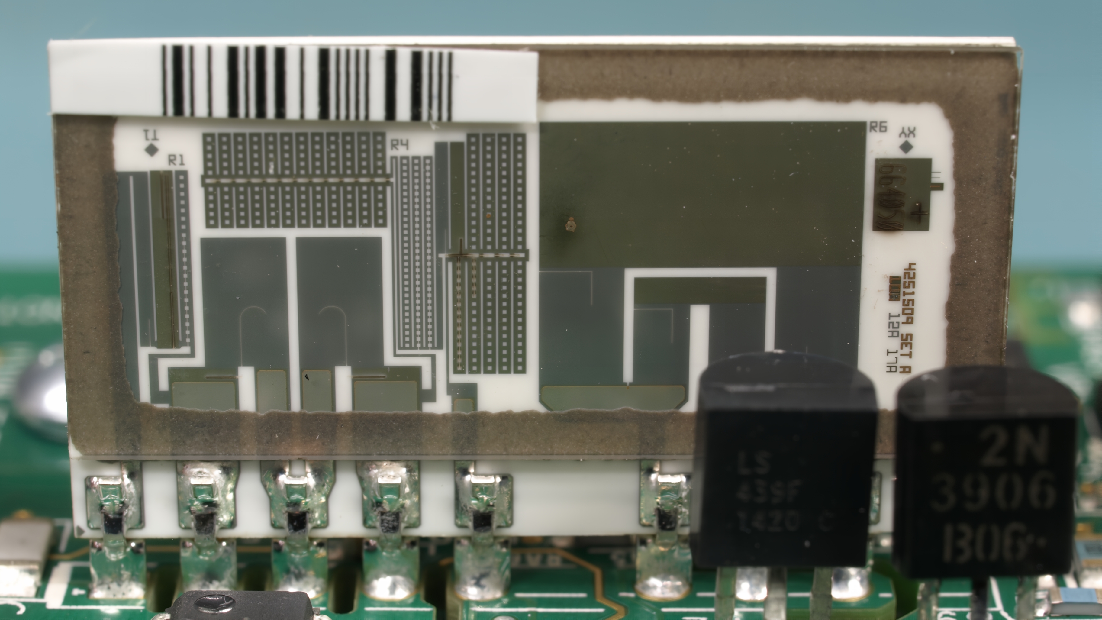
The practical consequence is the matched resistor network: two or more elements of the same material, deposited side by side on one substrate, laser-trimmed together, and packaged in one body so they share a temperature. A precision thin-film network can hold ratio tracking to a fraction of a ppm/°C even though each element’s absolute tempco is ten or twenty times larger. Two discrete 1% resistors from different reels, by contrast, might have tempcos that differ by 50 ppm/°C and sit at different temperatures on the board — their ratio wanders where the network’s holds rock-still. For anything that must keep a ratio — an instrumentation-amplifier gain set, a precision divider, a bridge — the matched network is the correct tool, and its datasheet leads with the tracking number for exactly this reason.

One more temperature effect closes the loop back to power. A resistor dissipating power heats itself above ambient, and that self-heating shifts its value through the very tempco just discussed. The value therefore depends, slightly, on how hard the part is being driven — a coupling between electrical operating point and resistance that a low-tempco part minimizes and a high-tempco part makes visible. In precision work the self-heating shift is a real error source, and it is one reason a designer running a resistor at a fraction of its rating buys not just longevity but stability.

3.4 Voltage coefficient: the value that moves with the volts

Less famous than tempco, and for that reason a more insidious trap, is the voltage coefficient of resistance (VCR): a small change in resistance with the voltage applied across the element, quoted in ppm per volt. It arises because the conduction mechanism in some resistive materials is not perfectly ohmic — the electric field within the element nudges the effective resistance, so a higher voltage produces a slightly different value than a lower one.

The effect is strongly type-dependent, and this is the key thing to remember. It is worst in thick-film resistors and in carbon composition, and worst of all in long high-voltage resistors, where a large potential is dropped across a physically extended element and the field per unit length is high. Thick-film VCR is often tens of ppm per volt; over a large voltage swing that is a measurable change in value. Metal-film and thin-film parts, by contrast, have negligible VCR — their conduction is close to ideally ohmic — and wirewound and foil parts are effectively immune.

Why does a few ppm per volt matter? Because it is a source of distortion. Consider a precision or audio voltage divider handling a swinging signal. If the resistance itself changes with the instantaneous voltage across it, the division ratio is no longer constant through the waveform — the divider is slightly nonlinear, and a pure sine wave emerges with a trace of harmonic content it did not have going in. In a high-resolution data-acquisition front end or a low-distortion audio stage this shows up as an error that no amount of tolerance-tightening fixes, because it is not a value error but a linearity error. The cure is to choose a material with low VCR (thin film, foil), to keep the voltage across any one element modest (in high-voltage dividers, this means using a series string of many resistors so each drops only a small fraction of the total), and to be suspicious of thick-film parts in any signal path where linearity is the specification.

3.5 The equivalent circuit: R is only the beginning

To account for the high-frequency behaviour, the resistor must be modelled not as a pure resistance but as a small network. The standard simplified model — the exact analogue of the ESR/ESL model for a capacitor and the DCR/inter-winding-C model for an inductor — is a resistance R in series with a small parasitic inductance L, the whole series pair shunted by a small parallel capacitance C.

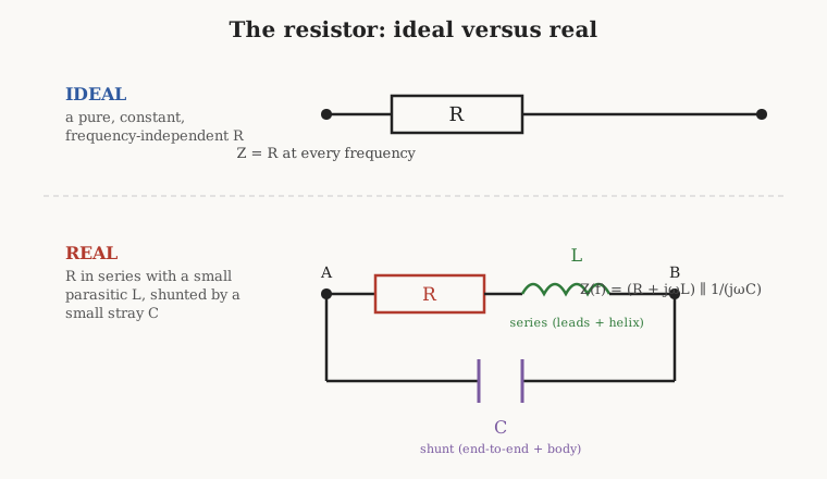
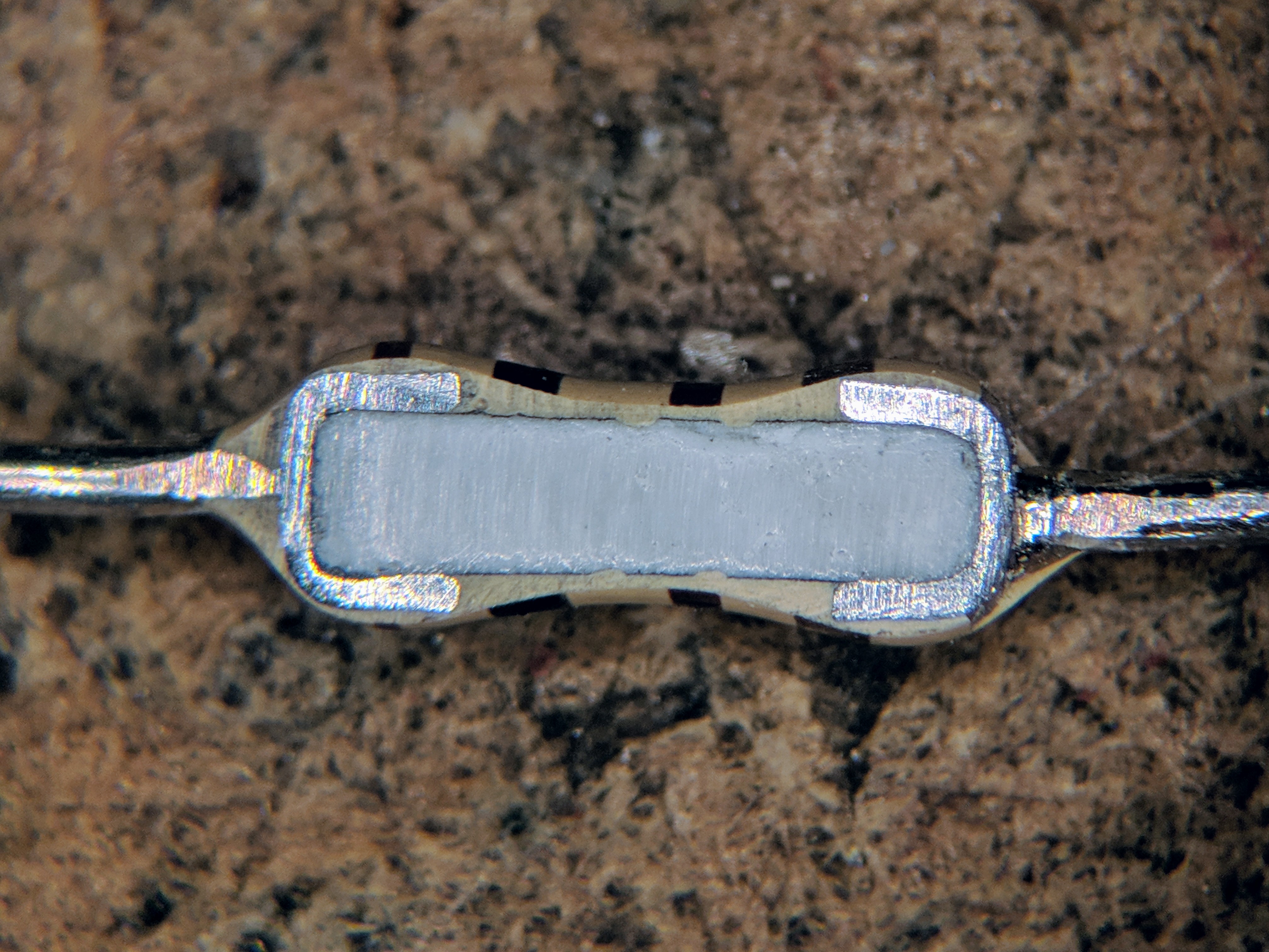
Each parasitic has a physical home. The series inductance L comes from two places: the leads (or the chip’s terminations and the traces feeding them), and — importantly — the helical path of the resistive element itself. Most film resistors reach their marked value by having a spiral groove cut into the film, turning a low-resistance cylinder into a long helical ribbon; that helix is, geometrically, a single-layer coil, and it has inductance for exactly the reason the coils in the sibling dive do. A wirewound resistor is even more obviously a coil, since it is a winding. The shunt capacitance C comes from the end caps facing each other across the body, from the distributed capacitance between adjacent turns of the film helix, and from the part to its surroundings. Neither parasitic is large — the L is typically a few to a few tens of nanohenries, the C a fraction of a picofarad to a couple of picofarads — but small is not zero, and at high frequency small reactances start to matter.

3.6 Frequency response: where the resistor stops being a resistor

From that equivalent circuit the frequency behaviour follows directly, and it splits by resistance value. The impedance the circuit presents is the series R-plus-L in parallel with the shunt C. At low frequency both reactances are negligible and the impedance is simply R — the flat, well-behaved region the schematic assumes. As frequency climbs, one of two things happens depending on whether the part is low-value or high-value.

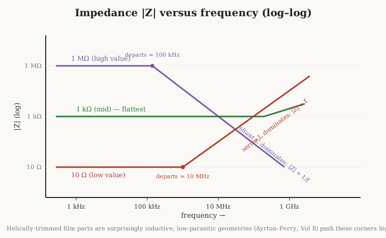
For a low-value resistor — say a few ohms to a few tens of ohms — the shunt C is irrelevant (its reactance stays enormous compared with the small R) but the series L eventually matters. Above a corner in the region of tens of megahertz to a few hundred megahertz, the inductive reactance ωL becomes comparable to R, and the impedance magnitude rises above the nominal value and gains a phase angle. The part looks partly inductive. This is why a “10 Ω” resistor used to damp a fast edge or terminate a line is not simply 10 Ω to the edge’s high-frequency content — and why helically-trimmed film parts, whose element is a literal coil, are “surprisingly inductive” and a poor choice where low parasitic L is essential.

For a high-value resistor — hundreds of kilohms to megohms — it is the other way round. The series L is trivial next to the large R, but the tiny shunt C provides a path that increasingly bypasses the resistance as frequency rises. Above a corner that can be as low as tens or hundreds of kilohertz for a megohm part, the shunt capacitance dominates and the impedance magnitude falls with frequency, ∝ 1/f, and the part looks partly capacitive. A 1 MΩ feedback resistor in a photodiode transimpedance stage, for instance, cannot be treated as 1 MΩ at high frequency; its shunt capacitance sets the bandwidth of the whole stage. Somewhere in the middle — around a kilohm or a few kilohms — sits the value where L and C most nearly balance and the impedance stays flattest longest; this is one quiet reason such mid-range values are so pleasant to design with.

The lesson the designer draws is that “non-inductive” construction and low-parasitic geometry are not marketing garnish but real, specifiable properties. The classic answer to the inductive-helix problem is the Ayrton–Perry winding — two counter-wound elements whose magnetic fields cancel — treated in the coming Volume 8; it, and the various low-inductance film patterns, exist precisely to push the inductive corner in Figure 6 up out of the band of interest. When a part is marked “non-inductive,” this is the deviation it is promising to have tamed.

3.7 Noise: the two hisses, and which one is the part’s fault

A resistor generates noise — a small, random, fluctuating voltage across its terminals — and there are two entirely different mechanisms at work. Confusing them is the source of a great deal of muddled thinking, so this section separates them cleanly. The first is unavoidable and identical for every resistor of a given value; the second is optional, depends on construction, and is the real quality differentiator between resistor types.

3.7.1 Thermal (Johnson–Nyquist) noise: the floor no one escapes

The first mechanism is thermal noise, also called Johnson–Nyquist noise after its discoverers. It arises from the random thermal agitation of the charge carriers inside any resistance; it needs no applied voltage and no current, and it is present the instant the resistor is above absolute zero. Its root-mean-square voltage over a bandwidth B is

Vn(rms) = √(4 · k · T · R · B),

where k is Boltzmann’s constant, 1.38×10⁻²³ joules per kelvin, T is the absolute temperature in kelvin, R the resistance in ohms, and B the bandwidth in hertz. The spectrum is flat — white noise — so it is often quoted as a spectral density in volts per root-hertz by setting B = 1 Hz.

The numbers are worth committing to memory as landmarks. A 10 kΩ resistor at room temperature (300 K), measured over an audio-ish bandwidth of 20 kHz, produces

Vn = √(4 × 1.38×10⁻²³ × 300 × 10 000 × 20 000) ≈ 1.8 µV rms.

The same resistor expressed as a spectral density — over a 1 Hz bandwidth — gives

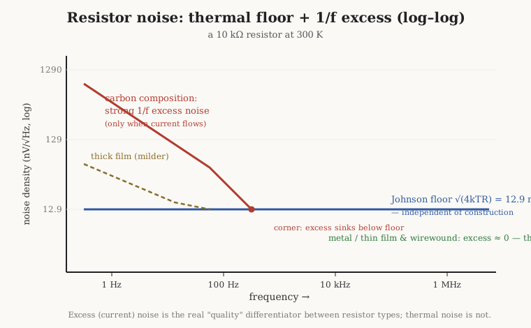
Vn = √(4 × 1.38×10⁻²³ × 300 × 10 000 × 1) ≈ 12.8 nV/√Hz.

Those two figures, ~1.8 µV in 20 kHz and ~12.8 nV/√Hz, are the fixed reference points for a 10 kΩ part. Because the voltage goes as the square root of R, a 1 kΩ resistor sits at about 4.1 nV/√Hz and a 1 MΩ at about 129 nV/√Hz. The crucial fact is what the formula does not contain: there is no term for the material, the construction, the brand, or the age. Thermal noise depends only on resistance, temperature, and bandwidth. A 10 kΩ carbon-composition resistor and a 10 kΩ bulk-foil resistor have identical thermal noise. This is the floor beneath every amplifier: the source resistance seen by an amplifier’s input sets a thermal-noise voltage that no amplifier, however quiet, can undo, which is why low-noise front ends favour low source impedances and why the resistor values around a sensitive input are chosen with the √R of this formula in mind.

3.7.2 Excess (current, 1/f) noise: the part’s own fault

The second mechanism is excess noise, also called current noise or 1/f noise, and it is a different animal entirely. It appears only when current flows through the resistor, it scales with that current (and with the applied voltage), and its spectrum is not flat but rises toward low frequency as roughly 1/f — so it dominates at DC and low frequencies and sinks below the thermal floor higher up. Physically it comes from the granularity of the conduction path: in a material where current threads through a jumble of conducting grains and contacts, the moment-to-moment conduction fluctuates, and those fluctuations, driven by the current, show up as an extra noise voltage on top of the thermal floor.

Because it is a property of the conduction path’s structure, excess noise depends enormously on construction — and this is where the resistor types finally separate on a noise basis. It is quantified by a noise index, given in microvolts of noise per volt of applied DC per decade of frequency (µV/V per decade). The ranking is stark. Carbon composition, whose current squeezes through a pressed mass of carbon granules and binder, is the worst — a high noise index, the reason vintage carbon-comp parts are audibly hissy in high-gain audio and unwelcome in any low-level DC-coupled stage. Thick film is middling — the conductive-particle-in-glass matrix has some granularity but far less. Carbon film sits between composition and metal. And metal film, thin film, and wirewound are near-zero — their conduction is through a continuous homogeneous metal, there is little granular structure to modulate, and their noise index approaches the theoretical floor. Bulk metal foil is likewise essentially excess-noise-free.

The contrast to hold onto is this: thermal noise is the same for all types and cannot be designed away (only cooled or reduced by lowering R or bandwidth); excess noise varies by orders of magnitude between types and is exactly what “resistor quality” means in a noise context. When a datasheet or a designer speaks of a “low-noise” resistor, it is the excess noise being praised — because the thermal noise was never anyone’s to improve. In a µV-level DC amplifier or a high-gain audio path, choosing metal or thin film over carbon composition is not audiophile superstition; it is the difference between a resistor that only contributes the unavoidable Johnson floor and one that piles a current-driven 1/f hiss on top of it.

3.8 Stability and drift: the value that ages

Tolerance describes the value at the moment of manufacture; stability describes how well the part holds that value over its working life, and it is a separate specification with its own physics. Several mechanisms slowly move a resistor’s value over months and years.

Load-life drift is the change after long operation at rated (or derated) power and temperature — a resistor that has dissipated its rated watts continuously for a thousand or ten thousand hours will have shifted, and the datasheet quotes the expected percentage as a load-life stability figure. Shelf life or aging is the slower change even in an unpowered part on a shelf, as the element and its terminations relax and equilibrate. Moisture intrusion changes the resistance of some elements, which is why humidity and the “damp heat” test appear in qualification, and why hermetic or well-encapsulated parts are specified where the environment is hostile. Thermal cycling — repeated expansion and contraction as the equipment heats and cools — stresses the element, the trim, and the terminations, and gradually shifts the value; it is a leading wear-out mechanism for chip resistors soldered to a board with a mismatched expansion coefficient.

There is also a subtle DC error that has nothing to do with the resistance value at all: thermal EMF. Wherever two dissimilar metals meet — the resistive element and its end cap, the end cap and the lead, the lead and the solder joint — a small thermoelectric voltage appears if the two junctions of the part are at different temperatures, on the order of microvolts per degree Celsius of junction-to-junction difference. In ordinary circuits this is invisible. In low-level DC instrumentation — a nanovolt-class amplifier, a precision reference divider — a few µV/°C of thermal EMF from a temperature gradient across a resistor is a real offset, and precision parts advertise a low thermal-EMF construction (symmetric terminations, matched metals) for exactly this reason. It is the resistor’s quiet contribution to the same family of problems that dogs precision connectors and switch contacts.

The composite figure that captures much of this is the part’s stability or long-term drift spec, often given in ppm or percent per 1000 hours or per year under stated conditions. For most work it can be ignored; for a voltage reference, a precision divider, or a calibration standard it is decisive, and it is the axis on which bulk metal foil — with drift measured in a few ppm over years — earns its considerable price over even good thin film.

3.9 Power derating: a preview

Everything above assumed the resistor was comfortably within its power rating. That rating is itself temperature-dependent, and it deserves a full treatment, which the coming Volume 9 provides. The essential idea to carry forward from here is simple: a resistor’s maximum allowed power dissipation is not a single number but a derating curve. The part can handle its full rated power only up to some ambient temperature (often 70 °C); above that, the permitted power falls linearly to zero at the maximum operating temperature (often 150 °C or higher), because the part’s own heat plus the ambient must not push the element past its limit. A resistor rated “0.25 W” in free air at 25 °C may be allowed only a fraction of that inside a hot enclosure. Running a part well below its derated limit is, as the self-heating discussion above showed, also the cheapest way to buy tempco stability and long load-life — which is why experienced designers habitually specify a power rating several times the expected dissipation. Volume 9 works the curves, the pulse and surge ratings, and the high-power packages in full.

3.10 The trade-space, by type

The deviations catalogued above do not vary independently; each resistor construction lands at a characteristic point across all of them at once, and choosing a type means choosing a combination of virtues and vices. The closing figure scores the common families — carbon composition, carbon film, metal film, thick film, thin film, wirewound, and bulk metal foil — on the five axes that this volume has developed: tolerance, tempco, voltage coefficient, excess noise, and parasitics. It is the same trade-space that the fixed-type Volumes 7 and 8 detail construction by construction; presented together here, it lets the reader see the whole landscape before descending into any one corner of it.

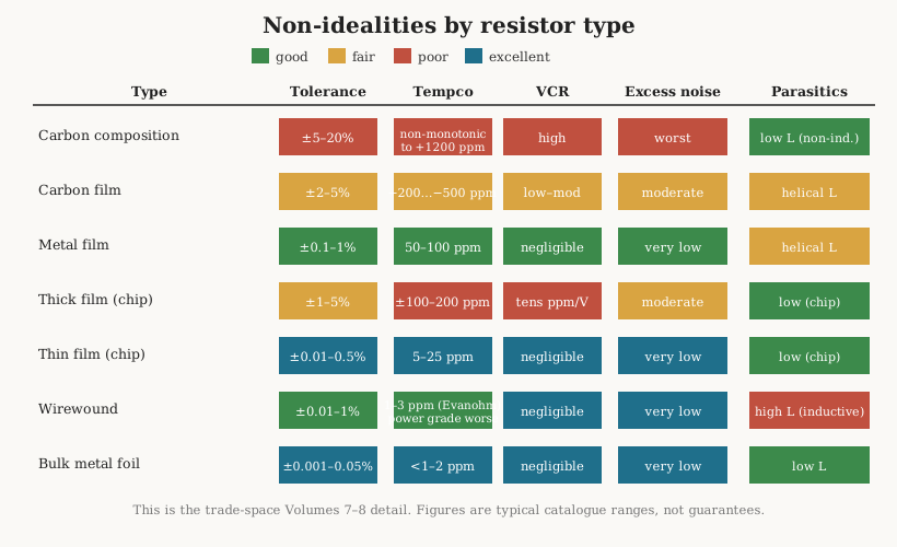
Reading the matrix reveals the logic of the market. Carbon composition is poor on almost every precision axis — loose tolerance, huge non-monotonic tempco, high VCR, the worst excess noise — yet it survives because its solid, non-helical body has low inductance and a large heat capacity, making it excellent at absorbing brief high-energy pulses; it is a pulse and surge part, not a precision part. Carbon film is the cheap general-purpose axial, better than composition on every count but still negative-tempco and noisier than metal. Metal film is the sweet spot for through-hole precision: tight tolerance, moderate tempco, negligible VCR, low noise, with only its helical inductance as a caveat. Thick film dominates surface-mount by sheer economy despite mediocre tempco and VCR, because for the vast majority of pull-ups, biases, and non-critical dividers those deviations do not matter and the price is unbeatable. Thin film is the precision surface-mount choice — excellent on every electrical axis, the material of matched networks and instrumentation. Wirewound offers superb tolerance, tempco, VCR, and noise for power and precision alike, at the cost of being the most inductive family of all — the reason the non-inductive windings of Volume 8 exist. And bulk metal foil sits at the apex of the precision axes — the lowest tempco, the best long-term stability, negligible VCR, low noise — the part a designer reaches for when the value must simply not move, and the budget allows it.

The reader now has the full picture of what separates the schematic symbol from the object on the bench. An ideal resistor is a single number; a real one is a number surrounded by a tolerance band, sliding with temperature and voltage, dressed in a little inductance and capacitance that carry it away from its value at high frequency, whispering a thermal hiss it cannot help and, in the cheaper types, a current-driven hiss it can, and drifting slowly over its life. Which of those deviations the designer must respect depends entirely on the job — but knowing that they all exist, and roughly how large each is for each type, is the difference between a circuit that works on the bench and one that keeps working in the field. The volumes that follow take each resistor family and each application in turn; this one has drawn the map of the ways a resistor can fail to be ideal, so that the rest of the dive can be read with those failures in mind.