The Real Transformer: Losses, Leakage, and Regulation

2.1 The part the ideal model leaves out

The foundational volume built the transformer up as an ideal object: two windings sharing a common magnetic flux, a voltage stepped exactly in the turns ratio, a current stepped inversely, an impedance reflected by the square of the ratio, and — crucially — not one milliwatt lost along the way. That is the right altitude for first understanding what a transformer does. A designer sketching a power supply reasons with the ideal transformer the way a mechanic reasons with a frictionless pulley: it captures the essential job and gets the arithmetic right. But no real transformer is frictionless. Plug an “ideal” 120 V–to–12 V transformer into the wall and measure the secondary with no load and you will read perhaps 13.5 V, not 12; hang the rated load on it and the reading sags to 12; press a fingertip to the case after an hour and it is warm, sometimes uncomfortably so. The warmth is energy that went in the primary and never came out the secondary. The sag is voltage that the turns ratio promised and the copper and iron quietly took back. Neither belongs in the ideal picture, and both are the subject of this volume.

This is the transformer’s version of a chapter every component in this program has earned. The Capacitors dive has its “real capacitor,” which takes the pure C apart into equivalent series resistance, leakage, and self-inductance. The Coils dive has its “real inductor,” with winding resistance, self-capacitance, self-resonance, and core saturation. The Resistors dive has its “real resistor,” with tolerance, temperature coefficient, noise, and parasitic reactance. This is the direct sibling of those chapters, and it gives the transformer’s non-idealities the same rigorous treatment: it takes the two-winding, flux-coupled component apart into every mechanism by which it strays from the textbook, assembles those mechanisms into a single equivalent circuit that a bench engineer can measure and compute with, and then reads the practical consequences straight off that circuit — the losses that become heat, the voltage that sags under load, the efficiency that peaks at a particular load and nowhere else, the surge of current at switch-on that trips breakers, and the whisper of noise that couples straight through the windings unless it is deliberately shielded.

The roadmap is the equivalent circuit. Everything in this volume is a named element in it. There are five deviations from the ideal, and the plan is to introduce each as a physical fact, draw it as a circuit element, and then read its consequence:

• Winding resistance — the copper is not a perfect conductor, so both windings have real ohms, and current through those ohms makes heat. This is the copper loss, and it rises steeply with load.
• Leakage inductance — not every line of flux threads both windings; some escapes into the air and links only one. That stray flux stores energy the way any inductor does, and it drops voltage under load.
• Magnetizing inductance — the core has finite permeability, so it takes a real current to magnetize it, even with nothing connected to the secondary. That current is mostly reactive and mostly constant.
• Core loss — dragging the iron around its magnetic cycle fifty or sixty times a second costs energy, through magnetic hysteresis and through eddy currents induced in the core itself. This is the iron loss, and it is present whenever the transformer is energized, load or no load.
• Inter-winding capacitance — the primary and secondary are two conductors separated by insulation, which is the literal definition of a capacitor. That small capacitance is invisible at 60 Hz but becomes a highway for high-frequency noise.

Assemble those five and the ideal transformer at the center is surrounded by parasitic hangers-on, exactly as the ideal capacitor, inductor, and resistor were in their own volumes. The rest of this volume builds that circuit piece by piece and then spends it.

2.2 Building the equivalent circuit, one element at a time

The standard way to reason about a real transformer is to keep the ideal transformer at the heart of the model — a perfect, lossless turns-ratio device — and to move every imperfection out of it into an external circuit element wired around it. This is a powerful bookkeeping trick: it lets the turns ratio stay clean and honest while every real-world blemish becomes a resistor or an inductor that can be measured, calculated, and, where possible, designed smaller. The result is the transformer equivalent circuit, one of the most useful diagrams in electrical engineering, and the money figure of this volume.

Start with the ideal transformer: primary winding with N₁ turns, secondary with N₂ turns, perfect coupling, no loss. Now add the imperfections in the order a real current meets them, flowing in from the primary terminals.

First, the primary winding resistance, called R₁. The primary is tens or hundreds of metres of enamelled copper wire wound onto a bobbin, and copper — as the Resistors dive established at length — has a real resistivity. That length of wire has real ohms, so R₁ appears in series with the primary, in the path of the incoming current. Likewise the secondary winding has its own resistance R₂, in series on the output side. These are just the DC resistances of the two coils, the numbers an ohmmeter reads across each winding, and they are the seat of the copper loss.

Second, the leakage inductance of each winding, called Lₗ₁ and Lₗ₂ (the subscript ℓ for “leakage”). In the ideal transformer, every line of magnetic flux produced by the primary threads through the secondary too — the coupling is perfect. In a real transformer it very nearly is, but not quite: a small fraction of the flux produced by the primary current loops back through the air (or through the core in a path that misses the secondary) and links only the primary. That stray, un-shared flux behaves exactly like the flux of an ordinary inductor wound on the primary alone, so it is modelled as a small inductance Lₗ₁ in series with R₁. The secondary has its own leakage inductance Lₗ₂ in series with R₂, from the flux that links only the secondary. Leakage inductance is the circuit fingerprint of imperfect coupling.

Third, and now stepping across the line rather than along it, the magnetizing branch. Even with the secondary open — nothing connected, no load current — a real transformer plugged into the mains draws a small current, because the core must be magnetized to set up the flux that makes the whole device work, and a core of finite permeability needs a real magnetizing current to reach a given flux. That current, being the current that establishes flux in an inductance, is modelled as a shunt (parallel) inductance across the primary called the magnetizing inductance, whose reactance at the operating frequency is written Xₘ. It is large — the magnetizing current is a few percent of full-load current in a decent design — but finite, and it is the circuit’s admission that the core is not infinitely permeable.

Fourth, wired in parallel with that magnetizing inductance, the core-loss resistance, called R_c (sometimes R_fe, “fe” for the Latin ferrum, iron). Magnetizing the core does not merely store energy in the field; it also dissipates energy every cycle, through hysteresis and eddy currents (both detailed below). Dissipation means a resistive element, and because this loss is driven by the voltage across the core — the same voltage that drives the magnetizing current — it is modelled as a resistance R_c in parallel with Xₘ. The two together form the magnetizing branch: R_c carries the small in-phase current that becomes iron loss, and Xₘ carries the larger quadrature current that magnetizes the core. Their parallel combination draws the transformer’s total no-load, or exciting, current.

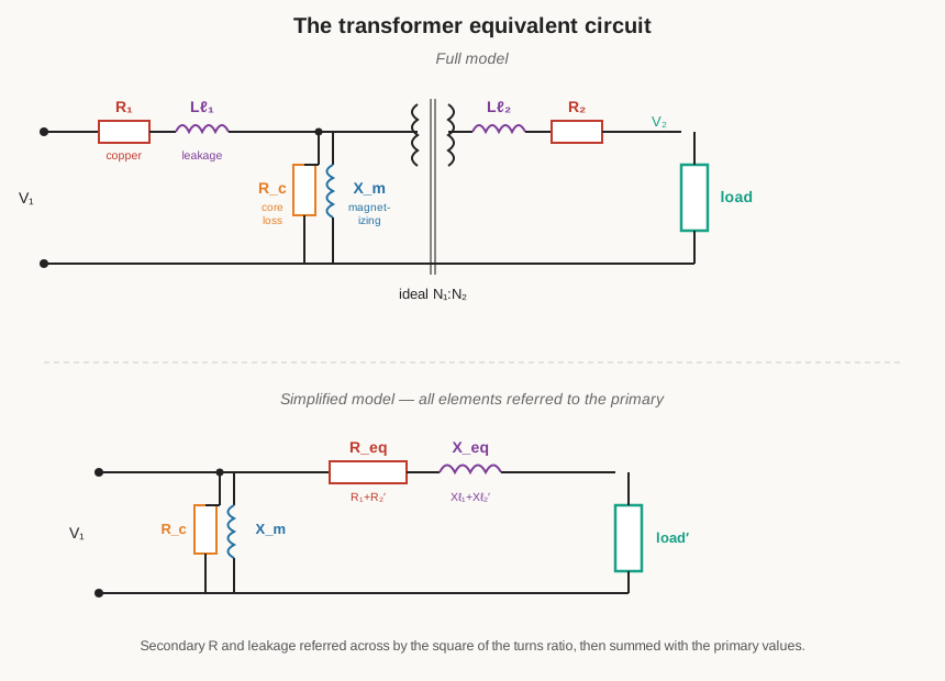
That is the full equivalent circuit, shown in the top half of Figure 1: R₁ and Lₗ₁ in series from the primary terminals, the shunt magnetizing branch (R_c ‖ Xₘ) across the line, then the ideal N₁:N₂ transformer, then Lₗ₂ and R₂ in series out to the load. Reading it left to right traces the fate of the incoming power: some current is peeled off by the magnetizing branch to feed the core (and its loss); the rest crosses the ideal transformer to the secondary, dropping voltage in the series resistances and leakage reactances on the way. Every non-ideality named in the roadmap is on this diagram, and the entire remainder of the volume is a tour of its elements.

2.2.1 Referring to one side: the simplified model

The full circuit is exact but awkward, because the secondary elements R₂ and Lₗ₂ live on the far side of the ideal transformer, at a different voltage and current level from the primary elements. Engineers routinely simplify it by referring all the elements to one side — usually the primary. Because the ideal transformer scales impedance by the square of the turns ratio (the N² reflection established in the foundational volume), a secondary resistance R₂ “looks like” R₂ × (N₁/N₂)² when viewed from the primary. Referring R₂ and Lₗ₂ across in this way, they can be added directly to R₁ and Lₗ₁, because now they are all on the same side of the (now-vanished) ideal transformer. The result is a single equivalent series resistance R_eq and a single equivalent series reactance X_eq, as shown in the bottom half of Figure 1.

A second, almost universal simplification moves the magnetizing branch out to the input terminals, ahead of the series elements. Strictly it sits after R₁ and Lₗ₁, but the voltage drop across those primary elements due to the tiny exciting current is negligible, so shifting the branch to the front introduces almost no error and makes the arithmetic far easier: the exciting current is now computed directly from the applied voltage, and the load current flows through one clean series R_eq + jX_eq. This “referred, approximate” equivalent circuit — a shunt magnetizing branch at the input, then a single series impedance to the load — is the workhorse model behind every calculation in this volume, and its two parameters are exactly what the open-circuit and short-circuit bench tests measure, a point the measurement volume develops in full.

2.3 Copper loss: the price of carrying current

The most intuitive loss is the one in the copper. Current flowing through the winding resistances R₁ and R₂ dissipates power as heat, at the rate every resistor obeys: P = I²R. The primary carries the primary current through R₁, the secondary carries the secondary current through R₂, and the total copper loss is the sum:

P_copper = I₁² · R₁ + I₂² · R₂

Two features of this loss govern everything about how a transformer is rated and how it behaves under load. First, it is proportional to the square of the current, and the current is proportional to the load. Double the load — draw twice the secondary current — and the copper loss quadruples. Run at half load and the copper loss falls to a quarter. Copper loss is therefore the load loss: near zero at no load, rising steeply as the transformer is worked harder, and reaching its rated value only at full rated current. This quadratic dependence is why a transformer comfortable at its nameplate rating overheats so quickly when overloaded — a 25 % overload raises the copper loss by more than 50 %.

Second, because R₁ and R₂ are the DC resistances of the windings, copper loss is a direct consequence of wire gauge and winding length, and it is the loss a designer trades against copper cost and window space. Thicker wire has lower resistance and lower copper loss but costs more, weighs more, and may not fit the bobbin window; thinner wire is cheaper and fits easily but runs hotter. The Coils dive laid out the wire-gauge and current-density arithmetic in detail, and it carries straight over: a transformer designer picks a current density — commonly on the order of a few amps per square millimetre for a naturally-cooled mains transformer — and sizes each winding’s wire accordingly, then lives with the copper loss that results. At elevated frequency there is a subtlety the DC resistance misses: skin effect and proximity effect crowd the current toward the conductor surface and raise the effective AC resistance above the DC value, so R₁ and R₂ in a switch-mode or RF transformer are the AC resistances, not the ohmmeter readings — which is why those transformers use fine stranded Litz wire or thin foil, again as the Coils dive develops.

2.4 Core loss: the price of magnetizing the iron

The second great loss lives not in the copper but in the iron, and it is present the moment the transformer is energized, whether or not any load is connected — which is why it is called the iron loss or no-load loss, and why leaving a transformer plugged in with nothing attached still costs energy and still makes the core faintly warm. Core loss has two distinct physical origins that add together: hysteresis loss and eddy-current loss.

2.4.1 Hysteresis: the reluctant iron

A transformer core is a ferromagnetic material — silicon steel, ferrite, or an amorphous alloy — full of microscopic magnetic domains. As the alternating primary current drives the flux up and down each cycle, those domains are dragged back and forth, forced to re-align first one way and then the other. They do not follow the driving field willingly; they resist re-alignment and lag behind it, so that the flux density B in the core traces out a loop rather than a single line as the magnetizing field H swings positive and negative. This is the famous B-H hysteresis loop, and its shape encodes the loss.

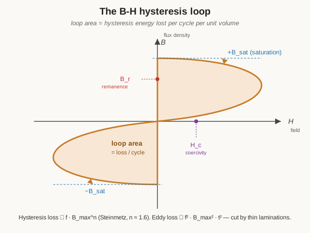
The key fact, shown in Figure 2, is that the area enclosed by the loop is the energy dissipated as heat, per cycle, per unit volume of core. A “fat” loop — a material with high coercivity, hard to demagnetize — wastes a lot of energy each cycle; a “thin,” narrow loop wastes little. This is exactly why transformer cores are made of magnetically soft materials engineered for the slimmest possible loop, while permanent magnets are made of magnetically hard materials with enormous loops. Because the loop is traversed once per cycle, the total hysteresis power is the loop area times the frequency. The relation the German-American engineer Charles Steinmetz distilled from measurement, and which still bears his name, captures it compactly:

P_hysteresis ∝ f · B_max^n

where f is the frequency, B_max is the peak flux density each cycle, and the exponent n — the Steinmetz exponent — is a material constant that runs from about 1.5 to 2.5 and is classically taken as roughly 1.6 for silicon steel. The lesson for a designer is severe: hysteresis loss climbs faster than linearly with how hard the core is driven, so pushing B_max up to save copper and iron (fewer turns, smaller core) is paid for by a more-than-proportional jump in hysteresis loss. It is a central tension in transformer design, and the design volume returns to it with the EMF equation in hand.

2.4.2 Eddy currents: the core as an unwanted secondary

The second half of the iron loss is subtler and, historically, the one that nearly killed the early transformer. The core is not only magnetic; it is also, if made of solid steel, an electrical conductor. The same changing flux that induces a useful voltage in the secondary winding also induces voltages within the core material itself, and those voltages drive swirling loops of current — eddy currents — circulating in the plane perpendicular to the flux. Those currents flow through the resistance of the core metal and dissipate power as I²R heat, exactly like a shorted secondary winding wrapped around nothing useful. A solid iron core would run ruinously hot and waste an enormous fraction of the input; the first practical transformers had to solve this before they could work at all.

The cure is lamination. Instead of a solid block, the core is built from a stack of thin sheets — laminations — each coated with a thin insulating oxide or varnish so it is electrically isolated from its neighbours, and the sheets are oriented parallel to the flux so they do not impede it. Slicing the core into thin insulated layers breaks up the large eddy-current loops into many small ones, each confined to one thin sheet, each enclosing far less flux and meeting far more resistance. The result is that eddy-current loss falls with the square of the lamination thickness:

P_eddy ∝ f² · B_max² · t²

where t is the lamination thickness. Halving the sheet thickness quarters the eddy loss. Mains-frequency power transformers use silicon-steel laminations typically 0.35 mm down to 0.23 mm thick; the silicon in the steel also deliberately raises its electrical resistivity to throttle the eddy currents further. Note the frequency dependence: eddy loss rises with the square of frequency, while hysteresis rises only linearly — which is why laminated steel becomes hopeless at high frequency and switch-mode transformers move to ferrite, a ceramic magnetic material that is a near-insulator and so has almost no eddy currents at all, or to ultra-thin amorphous ribbon. The Coils dive’s core-materials treatment carries over wholesale; Volume 4 of this dive develops the transformer-specific core geometry.

Crucially, core loss depends on the flux, and the flux is set by the applied voltage and frequency, not by the load. As long as the transformer is plugged into a fixed mains voltage, the peak flux B_max is essentially constant whether the secondary is open or fully loaded, so the core loss is essentially constant with load — the flat “iron loss” that sits underneath everything. That constancy, set against the load-rising copper loss, is what sets the efficiency curve, developed below.

2.5 Leakage inductance: the flux that got away

Return to the leakage inductances Lₗ₁ and Lₗ₂ and give them the physical picture they deserve, because leakage is the non-ideality with the widest reach — it sets voltage regulation, it limits high-frequency coupling, and in some transformer types it is deliberately engineered rather than merely minimized.

In the ideal transformer, all the flux is mutual flux: it circulates in the core and threads both windings, coupling them perfectly. In reality a small part of the flux produced by each winding takes a path that does not link the other winding — it bulges out of the core into the surrounding air, or takes a short-cut through the window, and returns without ever passing through the far coil. This is the leakage flux, shown in Figure 3.

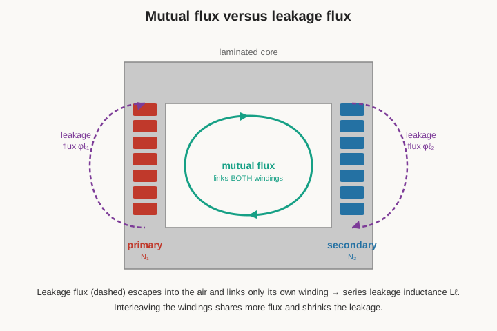
Because the leakage flux links only its own winding, it stores energy exactly as an ordinary inductor does and appears as the series inductance Lₗ in that winding — energy shuttled into the leakage field on each half-cycle and returned on the next, contributing no useful transfer to the secondary but dropping voltage along the way. The amount of leakage is a geometry problem: it depends on how the two windings are arranged relative to each other. Windings that are far apart — primary on one leg, secondary on the other — have high leakage; windings that are physically close and overlapping have low leakage. The standard technique to minimize it is interleaving: rather than winding the whole primary and then the whole secondary in separate concentric layers, the winder splits them into sections and sandwiches them — half the primary, then the secondary, then the other half of the primary — so the two windings are intimately intertwined and nearly all the flux is shared. Interleaving can cut leakage inductance dramatically, and the winding volumes of this dive treat exactly how it is done, layer by layer.

Leakage is not always the enemy, though. In some transformers it is a feature: the leakage reactance provides built-in current limiting (a welding transformer or a neon-sign transformer is deliberately built “leaky” so that a short on the output simply drives the leakage reactance and limits the current rather than exploding), and in resonant switch-mode converters the leakage inductance is used as a resonant element. The design volumes take up these deliberate-leakage designs; for now it is enough that leakage inductance is the circuit shadow of imperfect coupling, minimized by interleaving when it is unwanted and exploited when it is.

2.6 Magnetizing and exciting current: what the transformer draws at rest

Consider the transformer with its secondary open — no load at all — and ask what current it draws from the mains. In the ideal transformer the answer is zero: no load current, no primary current. The real answer is a small but non-zero current called the exciting current (or no-load current), and its makeup is instructive because it is the magnetizing branch of the equivalent circuit made visible.

The exciting current has two parts, corresponding to the two elements of the magnetizing branch. The larger part is the magnetizing current proper, flowing through Xₘ: the reactive current that sets up the alternating flux in the core. Being the current of a nearly pure inductance, it lags the applied voltage by close to 90° — it is almost entirely reactive, shuttling energy into the magnetic field on one quarter-cycle and pulling it back out on the next, doing no net work. The smaller part flows through R_c: the in-phase, real current that supplies the hysteresis and eddy-current losses — the core loss — and is dissipated as heat. Add them and the total exciting current is small (a well-designed mains transformer draws a no-load current of only a few percent of its full-load rating) and mostly reactive, dominated by the magnetizing component.

There is an important non-linearity hiding here. The magnetizing current is not a clean sinewave, because the core’s B-H relationship is not a straight line. As the flux approaches the material’s saturation flux density, the core permeability collapses — it takes disproportionately more magnetizing current to push the flux a little higher — so near the peak of each half-cycle the magnetizing current spikes upward and the waveform becomes sharply peaked and distorted, rich in odd harmonics (especially the third). This is why a transformer run at or above its rated voltage draws a magnetizing current that grows explosively with the last few percent of voltage: it is being pushed into saturation, where the exciting current can rise from a few percent to tens of percent of rated current for a small over-voltage. Designers therefore choose the operating flux density with a comfortable margin below saturation — a point the EMF-equation design volume makes quantitative — and the saturation behaviour is central to the inrush transient discussed below.

2.7 Regulation: why the voltage sags under load

Now the equivalent circuit pays its first practical dividend. Because the load current must flow through the series equivalent resistance R_eq and leakage reactance X_eq, it drops voltage across them, and that dropped voltage is subtracted from what reaches the load. The consequence is that the secondary voltage is higher at no load than at full load — the output sags as the transformer is worked — and the size of that sag is the transformer’s voltage regulation, defined as the fractional drop from no-load to full-load voltage:

Regulation (%) = (V_no-load − V_full-load) / V_full-load × 100 %

A transformer with good (low) regulation holds its output nearly constant from no load to full load; one with poor (high) regulation sags badly when loaded. The number matters enormously in practice: a nominal 12 V transformer with 15 % regulation actually delivers about 13.8 V unloaded and 12 V loaded, and a downstream circuit — a linear regulator, a relay coil, a lamp — has to tolerate that swing. Undersize the transformer and the regulation is poor and the rail sags; the classic symptom of an overtaxed supply is a voltage that droops the moment real current is drawn.

The physics of the sag is a phasor problem, because the drop across the series impedance has a resistive part (in phase with the current) and a reactive part (in quadrature), and how they add to the load voltage depends on the load’s power factor. Figure 4 shows the phasor construction: the full-load secondary voltage V_s is drawn as the reference, the load current I flows at some phase angle set by the load, and the voltage drops I·R_eq (along the current) and I·X_eq (at right angles to it) are added tip-to-tail. Their vector sum, added to V_s, gives the no-load voltage V_nl — visibly longer than V_s — and the difference between the two lengths, relative to V_s, is the regulation.

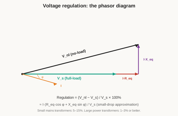
The diagram also shows the standard approximate formula that falls out of it for the usual case where the drops are small compared with V_s:

Regulation ≈ I · (R_eq·cos φ + X_eq·sin φ) / V_s

where φ is the load’s phase angle. At a purely resistive load (cos φ = 1) the resistive drop dominates; at a lagging (inductive) load the reactive drop I·X_eq adds substantially, which is why an inductive load worsens regulation and why leakage reactance matters as much as winding resistance. A worked case makes it concrete. Take a small mains transformer whose secondary, referred, has R_eq = 0.8 Ω and X_eq = 0.6 Ω, delivering 5 A at 12 V into a resistive load (cos φ = 1, sin φ = 0). The drop is I·R_eq = 5 × 0.8 = 4.0 V resistive plus 5 × 0.6 = 3.0 V reactive; the approximate regulation is 5 × (0.8 × 1 + 0.6 × 0) / 12 = 4.0 / 12 ≈ 33 % from the resistance alone — a deliberately poor example to show the mechanism. Realistic small mains transformers land in the 5 % to 15 % range; big power-grid transformers, built with far more copper and tighter coupling relative to their rating, achieve 1 % to 3 % or better. Regulation is the single most load-visible non-ideality, and it is set entirely by R_eq and X_eq — the copper and the leakage.

2.8 Efficiency: where the two losses cross

Combine the load-rising copper loss and the load-flat core loss and the transformer’s efficiency — output power divided by input power — follows a characteristic curve with a distinct peak. Efficiency is simply:

η = P_out / P_in = P_out / (P_out + P_copper + P_core)

At very light load, P_out is tiny but the core loss is still there in full, so efficiency is low — almost all the (small) input is being spent magnetizing the iron. As the load rises, P_out climbs while the core loss stays flat, so efficiency climbs quickly. But the copper loss is rising with the square of the load, and eventually it overtakes the benefit of more output; efficiency peaks and then slowly falls as copper loss dominates at heavy load. Figure 5 plots the three curves together: the flat core-loss line, the quadratically-rising copper-loss curve, and the resulting efficiency hump.

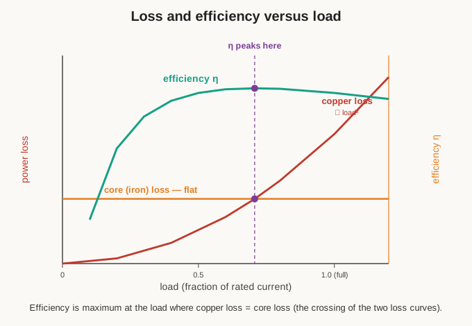
The peak sits at a mathematically clean and memorable place: efficiency is maximum at the load where the copper loss equals the core loss. This is not a coincidence but a direct consequence of the calculus — differentiating the efficiency expression with respect to load and setting it to zero gives exactly the condition P_copper = P_core. A designer who knows the fixed core loss can therefore choose the winding resistance so that the two losses are equal at the load the transformer will usually run at, placing the efficiency peak where it does the most good. A transformer that spends its life near full load is designed with copper loss equal to core loss at full load; a distribution transformer that idles most of the day at light load is deliberately designed with lower core loss (better steel, more of it) so that the peak sits at the low load it actually sees, since it pays that iron loss around the clock.

The numbers are worth anchoring. Small mains transformers — a few tens of watts — are typically 80 % to 90 % efficient at full load; the losses are a real fraction of the rating because the copper and iron do not scale down as favourably as the useful power. Efficiency improves with size: a several-hundred-watt toroidal transformer reaches the low-to-mid 90s, and large power-grid transformers, where every fraction of a percent is money burned continuously, achieve 99 % or better. All of the lost energy — copper loss and core loss alike — leaves as heat, which is why the ultimate limit on a transformer’s rating is not magnetic or electrical but thermal: how much loss it can shed before the winding insulation cooks. The design volume takes up temperature rise as the true rating ceiling.

2.9 Inrush: the surge at switch-on

There is one more current a real transformer draws that the equivalent circuit’s steady-state elements do not fully capture — a violent, transient one that lasts only a few cycles but can be ten to forty times the rated current: the inrush current at switch-on. Anyone who has seen the lights dim for an instant when a large toroidal amplifier is switched on, or had a breaker trip on power-up of an otherwise-innocent transformer, has met it.

The cause is a flux problem, not a load problem. In steady operation the core flux is a sinewave that lags the applied voltage by 90°, swinging between +B_max and −B_max. The magnetizing current that produces that flux stays small only because the flux stays within the core’s linear range. Now consider the worst-case switch-on: the mains happens to be switched on at the instant its voltage is passing through zero. From that starting point the flux, which is the time-integral of the voltage, does not swing symmetrically about zero — it builds in one direction for a full half-cycle before the voltage reverses, driving the peak flux toward twice the normal B_max. The core cannot hold twice its design flux; it saturates hard, its permeability collapses, and the only thing left to limit the current is the small winding resistance and leakage. The magnetizing current, freed from the saturated core’s inductance, spikes to an enormous first-cycle peak.

Worse, a transformer that has just been switched off may retain residual flux (remanence — the B_r marked on the hysteresis loop of Figure 2) frozen in its core. If the next switch-on happens to drive the flux in the same direction as the residual, the two add and the core is pushed even deeper into saturation, producing the very worst inrush. The magnitude therefore depends on both the switch-on phase angle and the leftover residual flux — a matter of luck on any given switching — which is why inrush is quoted as a worst-case multiple of rated current rather than a fixed number, and why the same transformer sometimes trips the breaker and sometimes does not.

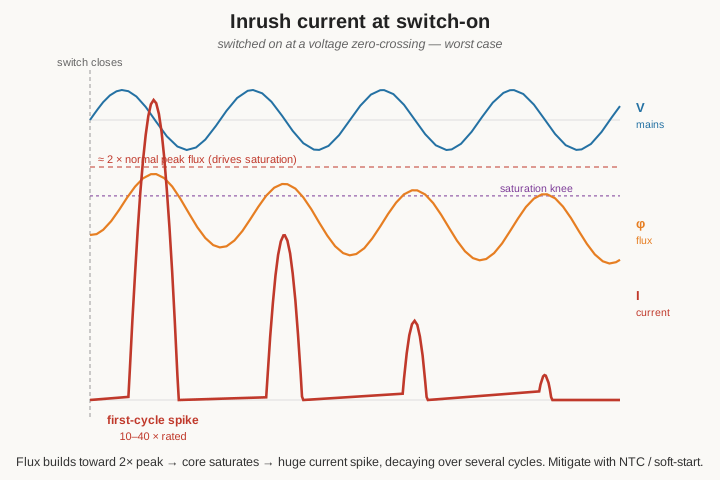
The mitigations all attack that first cycle. The simplest is a negative-temperature-coefficient (NTC) inrush limiter — a thermistor in series with the primary that is cold and high-resistance at the instant of switch-on, throttling the first surge, and then self-heats within a second or two to a low resistance so it wastes little power in normal running (a direct application of the NTC thermistor from the Resistors dive). More elaborate supplies use an active soft-start: a relay that initially inserts a series resistor and then, after a brief delay, shorts it out; or, in switch-mode supplies, controlled switching that ramps the flux up gently. Large transformers may use point-on-wave switching that deliberately closes the circuit at the voltage peak — the instant that produces a symmetric flux swing and the least inrush. Inrush is a transient the equivalent circuit predicts once its saturation non-linearity is admitted, and it is the reason transformer-input supplies need more than a bare fuse to survive their own switch-on.

2.10 Inter-winding capacitance and noise coupling

The final non-ideality is the one the low-frequency equivalent circuit ignores entirely and the high-frequency world cannot: capacitance. The primary and secondary windings are two sets of conductors separated by a thin layer of insulation — enamel, tape, bobbin wall. Two conductors separated by a dielectric are, by definition, a capacitor, so there is a small but real inter-winding capacitance between primary and secondary, and additional self-capacitance between the turns of each winding (the same winding self-capacitance the Coils dive analysed for the real inductor).

At 50 or 60 Hz this capacitance is invisible — its reactance is enormous and no meaningful current flows through it. But its reactance falls with frequency, and at high frequencies it becomes a low-impedance path that couples signal straight through the transformer, bypassing the magnetic coupling entirely. This defeats one of the transformer’s most valued jobs — galvanic isolation, the electrical separation of primary and secondary that the flux coupling provides while breaking any direct wire connection. For DC and mains frequencies the isolation is excellent, but high-frequency noise, and especially common-mode noise (interference that appears equally on both supply lines with respect to ground), rides across the inter-winding capacitance and past the isolation barrier as if the windings were wired together.

The cure is an electrostatic shield, also called a Faraday shield — a grounded conductive layer (a single turn of foil, or a winding of fine wire, deliberately not closed into a shorted loop so it carries no eddy current) placed between the primary and secondary. It intercepts the capacitive coupling: the stray capacitance now runs from the primary to the grounded shield, which shunts the high-frequency noise current to earth before it can reach the secondary, rather than from primary to secondary directly. A well-shielded isolation transformer can reduce inter-winding capacitance and common-mode coupling by orders of magnitude, which is why medical and instrumentation isolation transformers and the input transformers of sensitive audio and measurement gear are built with one or more Faraday shields. The shield costs a winding step and a ground connection and buys a large improvement in high-frequency isolation — a trade the types-and-design volumes return to for the transformers where noise rejection is the whole point.

2.11 The non-idealities, and which designs fight which

Every deviation in this volume is a handle a transformer designer can grasp, and much of the rest of this dive is the story of grasping them — choosing a core that fights core loss, a winding arrangement that fights leakage, a shield that fights capacitive noise, a size that fights regulation. The table below gathers the non-idealities, their circuit element, their consequence, and the design levers that combat each — a map of where the later volumes go.

Table 1 — The non-idealities, and which designs fight which

Non-ideality	Circuit element	Consequence	How designs fight it
Winding resistance	R₁, R₂ (series)	Copper (load) loss ∝ I²; heat; regulation	Thicker wire, lower current density, foil/Litz at HF (Vols 5, 9)
Leakage inductance	Lₗ₁, Lₗ₂ (series)	Voltage drop / regulation; limits HF coupling	Interleaved windings, toroidal & concentric geometry (Vols 4, 5, 11)
Magnetizing inductance	Xₘ (shunt)	No-load reactive current; saturation distortion	High-permeability core, adequate turns/flux margin (Vols 4, 6, 9)
Core loss — hysteresis	R_c (shunt)	Iron (no-load) loss ∝ f·B_max^n; constant heat	Soft, low-coercivity steel/ferrite; modest B_max (Vols 4, 9)
Core loss — eddy current	R_c (shunt)	Iron loss ∝ f²·B_max²·t²; constant heat	Thin laminations, silicon steel, ferrite at HF (Vols 4, 8)
Saturation	non-linear Xₘ	Distortion; inrush surge	Flux margin, gapping, point-on-wave / NTC / soft-start (Vols 4, 6, 9)
Inter-winding capacitance	C (parallel)	HF/common-mode noise breaches isolation	Faraday (electrostatic) shield, winding layout (Vols 5, 7, 8)

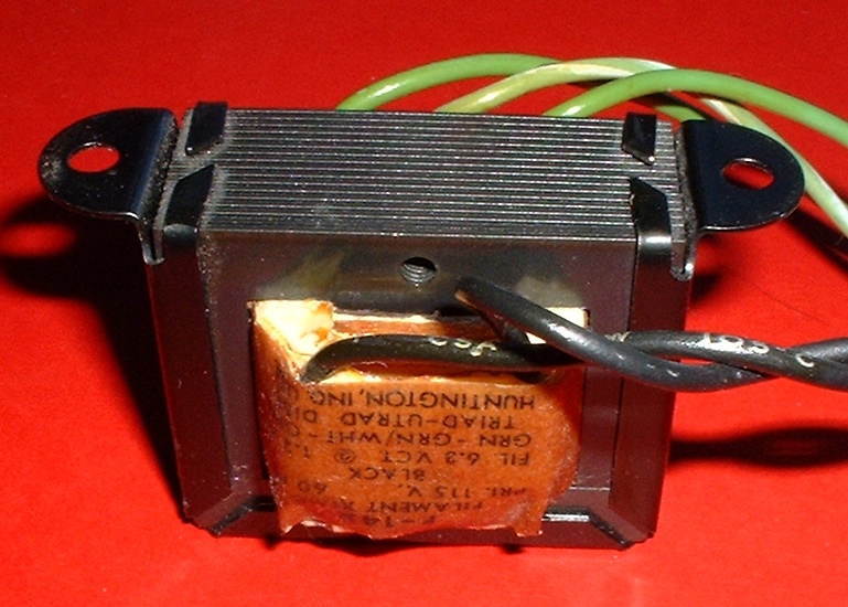
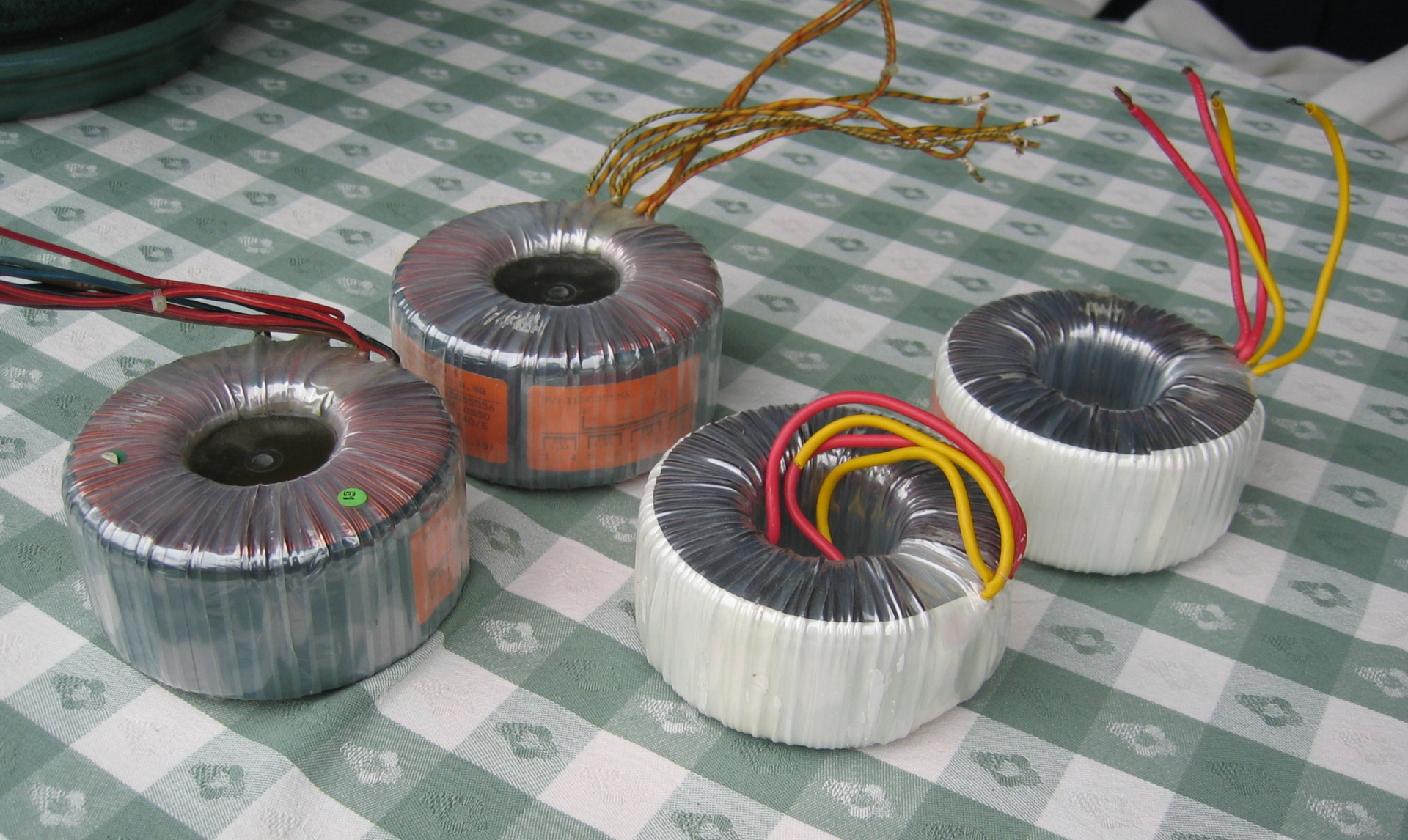
Read as a whole, the equivalent circuit is the transformer’s honest self-portrait: an ideal turns-ratio device at the center, ringed by the copper that carries the current, the leakage that escapes the core, the iron that must be magnetized and that fights being magnetized, and the capacitance that lets noise sneak past. Every real transformer the reader meets in the rest of this dive — the mains transformer, the toroidal, the tube output transformer, the current transformer, the flyback, the balun the reader may one day wind — is a particular set of compromises among exactly these elements. The photographs below show two of them made physical: the concentric windings and laminated core where copper loss, leakage, and core loss all live, and the seamless toroid whose closed magnetic path and tight winding give it the low leakage and low no-load loss that make it the quiet, efficient choice. The next volume steps back to the history that arrived at these designs; the volumes after it take the core, the wire, and the winding apart in the depth this program’s readers expect.