The Turns Ratio and Transformer Action in Depth

6.1 The one sentence that unlocks the whole component

Volume 1 introduced the transformer as a device that trades voltage for current at a ratio fixed by its turns: wind twice as many turns on the secondary as on the primary and the secondary voltage doubles while its current halves. That description is correct, and for a great many purposes it is enough. But it is a description of what a transformer does, not of why it does it, and the “why” is where every practical question — inrush, saturation, the buzz of an under-frequency core, the way an amplifier’s output transformer matches a valve to a loudspeaker, why the thing does nothing at all on a battery — is answered. This volume takes the ideal turns ratio of Volume 1 apart and rebuilds it from the physics, so that the reader leaves not with a formula to memorise but with a working mental model that predicts the machine’s behaviour on sight.

That model rests on a single sentence, and it is worth stating before anything else because everything downstream is a consequence of it: the magnetic flux in a transformer’s core is set by the voltage applied to the primary and by the frequency, not by the load. A transformer plugged into the mains runs at essentially the same core flux whether its secondary is open-circuit or delivering its full rated current. The load changes the current the windings carry, and it changes the small voltage droop called regulation, but it does not change the flux swinging around the iron. Hold that sentence firmly and the rest of the subject falls into place; lose it and transformer behaviour looks like a bag of unrelated tricks. The engineer who has internalised it can glance at a nameplate and know why a 120-volt primary on a given core needs the number of turns it does, why the same core saturates if fed 50-hertz power it was designed to see at 60, and why running the primary from anything with a direct-current component is asking for trouble.

6.2 Volts per turn: the flux is forced by the applied voltage

The physics is Faraday’s law, carried in full in Volume 3 and recalled here in the one form that matters for a transformer. A coil of N turns linking a changing flux Φ develops across its ends a voltage equal to the number of turns times the rate at which the flux changes: v = N · dΦ/dt, the “counter-EMF” or back-voltage. Now turn that around. The primary winding is connected across the supply. Ignoring for a moment the small winding resistance, the winding must develop a back-EMF that at every instant equals the applied voltage — if it did not, the tiny primary resistance would see an enormous net voltage and an impossible current would flow. So the applied voltage forces the winding to produce a matching back-EMF, and the only way the winding can produce that back-EMF is to have a flux changing through it at exactly the rate dΦ/dt = v / N. The applied voltage, in other words, dictates the rate of change of flux; integrate that rate over time and it dictates the flux itself.

For a sinusoidal supply this integration gives the single most-used equation in transformer work, the transformer EMF equation:

Vrms = 4.44 · f · N · Bmax · Ac

Here Vrms is the root-mean-square (the meter-reading) voltage across the winding, f is the frequency in hertz, N the number of turns, Bmax the peak flux density in the core in tesla, and Ac the cross-sectional area of the core in square metres. The curious constant 4.44 is not a fudge factor: it is 2π/√2, the number that appears when a sinusoidal flux is differentiated to give a voltage (that is where the 2π comes from) and the peak result is converted to an RMS value (that is where the √2 comes from). It is exact for a pure sine wave and only approximate for distorted waveforms.

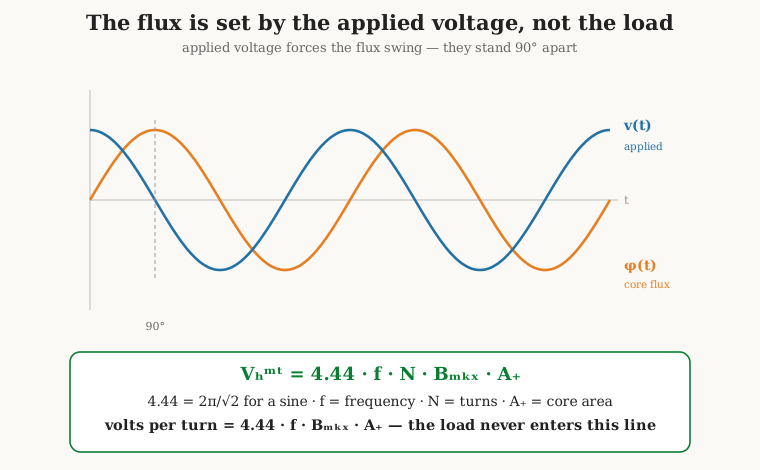
Read the equation as a statement about what is fixed and what is free. On the mains, Vrms and f are handed to the transformer by the utility and are not the designer’s to choose. Ac is set once the core is bought. That leaves Bmax — and the equation says Bmax is now fully determined: it is whatever value makes the arithmetic balance. The flux density adjusts itself to whatever the applied voltage and frequency require. The load is nowhere in the equation. This is the algebraic face of the opening sentence.

The most useful way to carry the equation on the bench is to divide out the turns and speak of volts per turn:

volts per turn = 4.44 · f · Bmax · Ac

Every winding on the same core — primary, secondary, a dozen taps — shares the same volts-per-turn figure, because they all link the same flux. This is the quantity the winder actually works with, and Volume 9 makes it the spine of transformer design. A worked number makes it concrete. Take a modest mains transformer with a core cross-section of 12 square centimetres (0.0012 m²) of silicon steel, worked at a peak flux density of 1.2 tesla, on a 50-hertz supply. The volts per turn are 4.44 × 50 × 1.2 × 0.0012 ≈ 0.32 volts per turn. A 230-volt primary therefore needs about 230 / 0.32 ≈ 720 turns; a 12-volt secondary needs about 12 / 0.32 ≈ 38 turns (a practical winder adds a few percent to the secondary to offset regulation, a point returned to below). Notice what the calculation did not require: any knowledge of the load. The turn counts are fixed by the voltages, the frequency, and the core — nothing else. That is the flux-set-by-voltage insight cashed out as a design.

6.3 Ampere-turn balance: how the primary “knows” to draw the current

If the flux does not depend on the load, a fair objection arises: how does the primary “know” to draw more current when a lamp is switched on across the secondary? The wall socket has no idea what is happening on the far side of the iron. The answer is the second pillar of transformer action, and it is as elegant as the first.

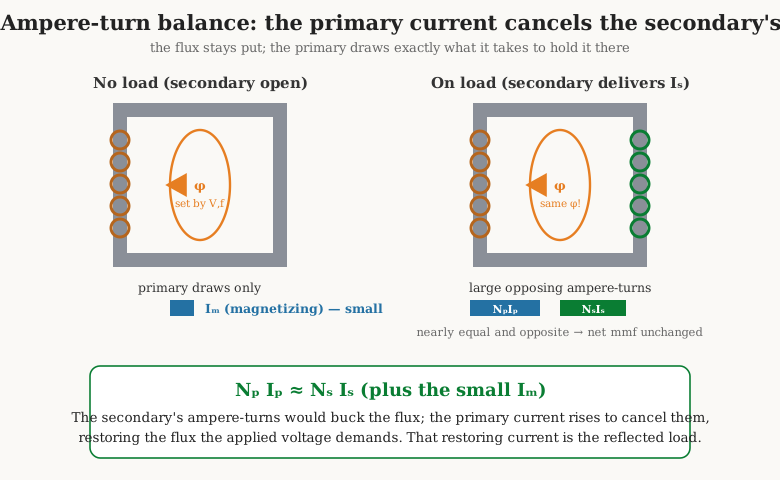
Consider the transformer at no load, secondary open. A small alternating current — the magnetizing current — flows in the primary and sets up the alternating flux the applied voltage demands. Nothing else happens; no power leaves the secondary because no current can flow in an open circuit. Now close the secondary onto a load. Current Is begins to flow in the secondary, and by Lenz’s law that current opposes the change that produced it: the secondary’s ampere-turns, Ns · Is, act to reduce the core flux. But the flux is not free to reduce — the applied primary voltage is still demanding exactly its old value, per the EMF equation. For an instant the flux does dip a hair; that dip lowers the primary’s back-EMF; the lowered back-EMF no longer balances the applied voltage; and the resulting net voltage drives additional current into the primary. That extra primary current, Ip, keeps rising until its ampere-turns Np · Ip exactly cancel the secondary’s demagnetizing ampere-turns and the flux is restored to the value the supply insists upon. The system self-corrects in a fraction of a cycle.

The steady-state result is the ampere-turn balance, the current counterpart of the voltage ratio:

Np · Ip ≈ Ns · Is

The primary and secondary ampere-turns are nearly equal and opposite; their fields very nearly cancel, leaving only the tiny net magnetomotive force needed to sustain the flux. This is precisely why the current ratio is the inverse of the voltage ratio — the step-up-in-voltage winding is the step-down-in-current winding — and it is the mechanism behind the power bookkeeping of Volume 1: volts up and amps down in the same proportion means volts-times-amps, the apparent power, passes through essentially unchanged. The primary does not “know” the load in any informational sense. It responds to a physical imbalance in the flux, and the imbalance is created the instant the secondary draws current. The transformer is a flux servo, and ampere-turn balance is its feedback law.

The word “approximately” in the balance is doing honest work. The two ampere-turns do not cancel perfectly; a small residue must remain, because some magnetomotive force is needed to drive the flux around the core’s reluctance. That residue is the magnetizing current, which the next section examines. The larger the load, the more completely the load-driven ampere-turns dominate that fixed magnetizing residue, which is why the balance equation is nearly exact at full load and only roughly true near no load.

6.4 The magnetizing branch: what flows when nothing is connected

At no load the transformer is not idle. It draws a small current — the exciting current, typically a few percent of the full-load primary current for a mains transformer, and less for a good toroidal one — whose job is to magnetize the core. Volume 2 built this into the equivalent circuit as the magnetizing branch, a shunt element across the primary, and split it into two parallel parts: a magnetizing inductance Lm that carries the reactive current setting up the flux, and a core-loss resistance Rc that represents the real power burned as hysteresis and eddy-current heating every cycle. The exciting current is the sum of a large reactive (magnetizing) component that lags the voltage by nearly 90 degrees and a small in-phase (loss) component that pays for the core heating.

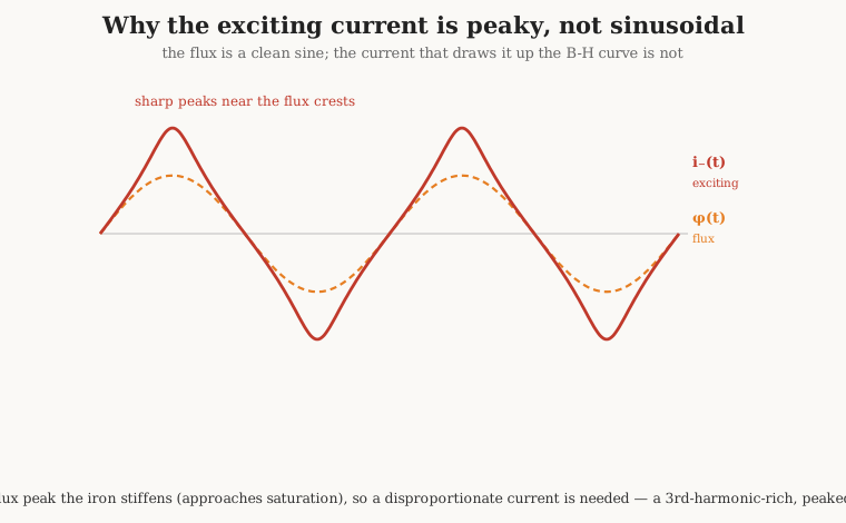
There is a subtlety here that the flux-set-by-voltage picture makes clear: the exciting current is not sinusoidal even when the flux is. Because the flux is forced to be a clean sine by the sinusoidal applied voltage, and because the relationship between flux density B and the magnetizing field H (hence the current) is the non-linear B–H curve of the iron treated in Volume 4, the current required to trace out that sinusoidal flux is distorted — sharply peaked near the flux crests, where the iron begins to stiffen as it approaches saturation. The exciting current of a mains transformer is rich in third harmonic for exactly this reason, and that harmonic content is one source of the transformer’s audible hum and of harmonic currents injected back into the supply.

The practical upshots are several. First, the exciting current sets the transformer’s no-load loss — the watts it burns doing nothing useful, which matter enormously for a distribution transformer energised twenty-four hours a day and hardly at all for a bench supply switched off at night. Second, the magnetizing inductance is the element measured by an open-circuit test (Volume 13): apply rated voltage to one winding, leave the other open, and the small current and the real power drawn give Lm and Rc directly, because with no load current the copper losses are negligible and nearly all the measured power is core loss. Third, and most important for the mental model, the magnetizing current is the “residue” of the ampere-turn balance made visible: it is the ampere-turns the primary must supply over and above those that cancel the secondary, the price of pushing flux through a core of finite permeability. A perfect core would need none.

6.5 Impedance reflection: the load seen through the ratio, squared

Because the transformer scales voltage by the turns ratio n = Np*/N*s and current by its inverse, it scales impedance — the ratio of voltage to current — by the ratio squared. A load Zs hung on the secondary appears at the primary terminals as

Zp = (Np / Ns)² · Zs = n² · Zs

Volume 1 introduced this as the “N-squared trick”; here it earns its keep. The squaring follows directly and inevitably: primary voltage is n times secondary voltage, primary current is 1/n times secondary current, so their ratio — the impedance the source sees — is n times 1/(1/n) = n² times the secondary’s ratio. The transformer is, seen from its input, an impedance transformer as much as a voltage transformer, and in a great many applications that is the entire point of using one.

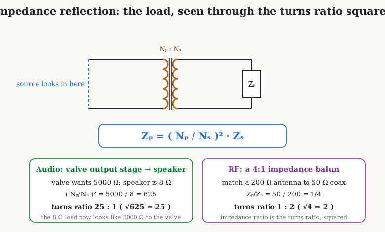
Two classic cases show the reach of the idea. The first is the valve (vacuum-tube) audio output transformer, examined as a type in Volume 7. A power valve is a high-voltage, low-current device; it delivers its power most efficiently and with least distortion into a load of several thousand ohms — a single-ended triode might want 3,000 to 5,000 ohms as its plate load. A loudspeaker is a low-voltage, high-current device of perhaps 8 ohms. The two cannot be connected directly without crippling the valve, and the output transformer exists solely to bridge the impedance chasm. To make an 8-ohm speaker look like 5,000 ohms, the turns ratio must satisfy n² = 5,000 / 8 = 625, so n = 25; a 25-to-1 step-down transformer presents the valve with the plate load it wants while delivering current-heavy, voltage-light drive to the speaker. Nothing about the voltage the speaker needs sets this ratio — it is chosen entirely to reflect the right impedance back to the valve. This is impedance matching, and it is the transformer’s oldest job after voltage changing.

The second case is radio-frequency matching, the province of Volume 8. A transmitter’s output stage or a length of coaxial cable expects a specific characteristic impedance — 50 ohms is the near-universal RF standard — while an antenna or a mixer or a following stage presents something else. A transformer wound as a balun or unun reflects one to the other. To match a 200-ohm folded-dipole feed to 50-ohm coax, the required impedance ratio is 200 / 50 = 4, so the turns ratio is √4 = 2: a 2-to-1 transformer is a “4-to-1 balun,” named by its impedance ratio in the RF tradition rather than its turns ratio. The same squaring law that sizes a valve amplifier’s output transformer sizes a shortwave antenna’s matching transformer; only the frequencies and the construction differ.

Impedance reflection also explains a fact that puzzles newcomers: a transformer’s own leakage inductance and winding resistance, referred from one side to the other, transform by n² as well. A tenth of an ohm of secondary resistance on a 25-to-1 output transformer appears at the primary as 0.1 × 625 = 62.5 ohms, which is why the copper losses of the low-turns, heavy-current winding are not negligible when reflected into the high-impedance side. The equivalent circuit of Volume 2 is built on exactly this referral.

6.6 From no load to full load: what actually changes

Armed with the flux-set-by-voltage rule and ampere-turn balance, the transformer’s behaviour as load is applied is now fully predictable. The flux barely changes — it is pinned by the applied voltage and frequency. The primary current rises, tracking the secondary current through the ampere-turn balance, from the small exciting current at no load to the full reflected load current plus that exciting residue at full load. The secondary voltage sags a little, and that sag is the one genuinely load-dependent voltage in the machine.

That sag is regulation, developed at length in Volume 2 and named here only to place it in the mechanism. It arises not from any change in flux but from the ohmic and reactive voltage drops in the windings themselves: as load current flows, it drops voltage across the primary and secondary winding resistances (copper loss) and across the leakage inductance (the flux that fails to link both windings), so the voltage that actually appears at the secondary terminals is a few percent below the ideal turns-ratio value. A transformer with 4 percent regulation delivers, at full load, a secondary voltage 4 percent below its no-load value. This is why the winder above added turns to the 12-volt secondary: to hit 12 volts under load, the winding must read a little high at no load. Regulation is a property of the real, lossy transformer; the ideal transformer of Volume 1 has none, because it has no winding resistance and no leakage. The flux, throughout, is a near-constant — the small droop in terminal voltage is not a droop in core flux but a drop across the series impedance between the core and the terminals.

The corollary matters for anyone sizing a supply: a transformer’s apparent-power rating in volt-amperes is a thermal rating, set by how much winding current the copper can carry and how much core and copper heat the assembly can shed before its insulation cooks (the temperature-rise budget of Volumes 5 and 9). It is not a flux limit. The core sits at the same flux at no load and full load; what fills up at full load is the current-carrying capacity of the wire and the heat budget of the whole structure.

6.7 Why alternating current only, and how direct current kills it

The flux-set-by-voltage rule, taken to its logical end, explains the transformer’s single most conspicuous limitation: it does nothing on steady direct current. Volume 1 stated the fact; the mechanism is now plain. The secondary voltage comes from dΦ/dt, the rate of change of flux. A steady DC applied to the primary produces, after the initial switch-on transient dies away, a steady flux — and a steady flux has dΦ/dt = 0, so the secondary voltage is zero. Connect a battery across a transformer primary and, once the brief turn-on surge has passed, the secondary is dead. Worse, with no back-EMF to oppose it (the winding produces back-EMF only from changing flux), the DC is limited only by the winding’s small resistance, so the primary draws a large steady current that simply heats the copper. A transformer on DC is an expensive resistor with a fire risk. Only a changing magnetic field induces a secondary voltage, and only alternating current — or switched, pulsed, or otherwise time-varying current — provides one. This is not a defect to be engineered away; it is the defining physics of the device.

A more insidious problem is a DC component riding on an AC waveform — a half-wave rectified feed, an unbalanced push-pull output stage, a Hall-effect current sensor’s bias, or simply an asymmetry in the driving electronics. The AC part transforms normally, but the DC part has nowhere to go: it drives a steady magnetizing current that adds a fixed offset to the flux. Because the AC flux swings symmetrically about zero in a well-behaved transformer, a DC offset shifts that whole swing toward one saturation limit, so on every positive half-cycle the flux is driven closer to — and eventually past — the saturation knee. The core, biased toward saturation half the time, draws huge current spikes on those half-cycles, heats, and hums. This is why the DC balance of a transformer’s drive matters so much, and why several transformer families are built specifically to tolerate or exploit DC. Push-pull and center-tapped output stages are arranged so that the DC magnetizing forces of the two halves cancel in the core, leaving it DC-free. Flyback and other DC-biased converter transformers (Volume 8) deliberately store energy in a gapped core, and the air gap — treated in Volume 4 — shears the magnetization curve over so that a substantial DC bias can be tolerated before the core saturates, at the cost of a higher magnetizing current. The gap is, in effect, a shock absorber for DC.

6.8 Saturation and the flux ceiling

The core cannot carry unlimited flux. Every magnetic material has a saturation flux density, Bsat, beyond which its magnetic domains are as aligned as they will ever be and the material carries no more flux however hard it is driven — for grain-oriented silicon steel about 1.9 to 2.0 tesla, for a manganese-zinc power ferrite only 0.4 to 0.5 tesla, as tabulated in Volume 4. Below that ceiling the core is a willing flux conductor, needing only a small magnetizing current to reach a given flux; approach the ceiling and the iron stiffens, its effective permeability collapsing toward that of air, so that a small further increase in flux demands an enormous increase in current. That collapse is the saturation knee, and crossing it is the transformer engineer’s cardinal sin.

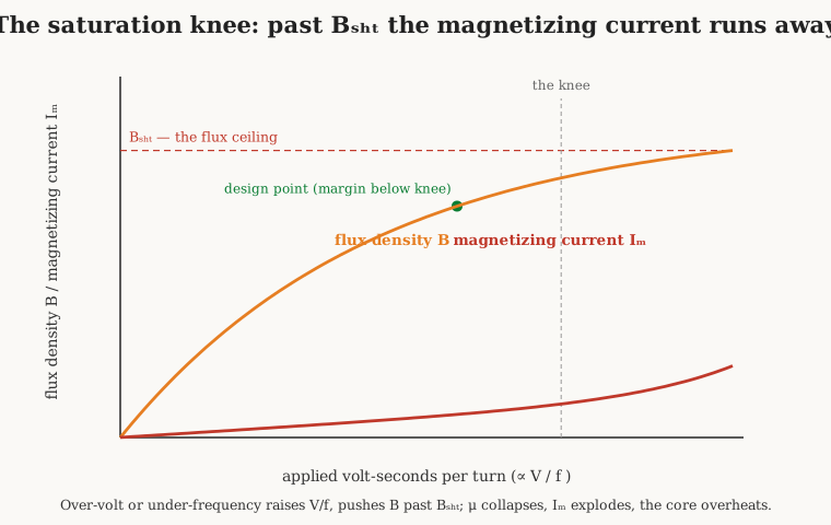
The EMF equation says when a transformer saturates. Rearranged, Bmax = Vrms / (4.44 · f · N · Ac). The flux density rises if the applied voltage rises, or if the frequency falls — both increase the “volt-seconds per turn” the core must absorb each half-cycle. Push Vrms too high (an over-voltage on the mains, a regulation fault, a lightning surge) or f too low (feeding a 60-hertz transformer with 50-hertz power) and Bmax climbs past Bsat. Once over the knee, the magnetizing inductance falls away, the exciting current no longer merely peaks but explodes into tall, narrow spikes many times the rated current, the voltage waveform flat-tops as the winding can no longer produce enough back-EMF, and the wasted magnetizing power heats the core. A saturated mains transformer draws heavy current, buzzes loudly, runs hot, and if the condition persists, burns out. The switch-on inrush surge of Volume 2 is a transient visit to exactly this regime: switching on at the wrong point in the cycle can drive the flux to nearly twice its normal peak before the steady state settles, momentarily saturating the core and drawing the well-known ten-to-forty-times-rated first-cycle current spike.

The defence is design margin. The mains-transformer designer, whose steel could reach 2.0 tesla, deliberately works it at a peak design flux of only 1.2 to 1.7 tesla, as Volume 4 laid out, leaving headroom for high line voltage, low line frequency, elevated temperature (which lowers Bsat), and the inrush transient. The margin is not timidity; it is the difference between a transformer that runs cool for decades and one that saturates on the first hot day when the utility voltage runs high. Ferrite designers, working from a much lower Bsat, leave proportionally similar margins and must watch Bsat fall with temperature especially closely, because a ferrite’s saturation flux density drops markedly as it warms toward its Curie point.

6.9 Frequency: 50 versus 60 hertz, 400 hertz, and the switch-mode kilohertz

Frequency appears in the EMF equation on an equal footing with voltage, and its effects are among the most practically important the volume covers. Everything follows from reading Bmax = Vrms / (4.44 · f · N · Ac): for a fixed voltage and turns, flux density is inversely proportional to frequency.

The classic trap is running a transformer below its design frequency. A transformer designed and rated for 60-hertz North American power, connected to a 50-hertz European supply at the same voltage, sees its core flux rise by the ratio 60/50 = 1.2 — a 20 percent increase. A core worked at, say, 1.5 tesla on 60 hertz now runs at 1.8 tesla on 50 hertz, uncomfortably close to or past the knee, and the symptoms are the classic saturation ones: excess magnetizing current, overheating, and audible buzz. The reverse — a 50-hertz transformer run on 60 hertz — is harmless as far as flux goes, because the flux falls by 50/60, leaving the core further from saturation; the only penalty is slightly higher winding impedance. This asymmetry is why “50/60 Hz” universal-input equipment is designed to the worst case, the 50-hertz flux, and why a transformer salvaged from 60-hertz gear should never be assumed safe on 50-hertz mains without checking its flux margin.

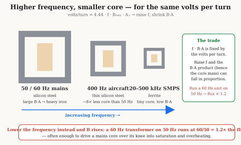
Run the logic the other way and it explains why high-frequency transformers are small. The product f · Bmax*· Ac is fixed by the volts per turn a design needs. Raise the frequency and, for the same volts per turn, the Bmax· A*c product can fall in proportion — which means the core can carry less flux, hence be built of less iron, hence be smaller and lighter. This is the entire reason aircraft power systems run at 400 hertz rather than 50 or 60: at nearly seven times the frequency, transformers and motors can be roughly that much smaller and lighter, and weight is everything in an aircraft. It is also why switch-mode power supplies, which chop their input into pulses at tens to hundreds of kilohertz before transforming it, use transformers a fraction the size and weight of a 50-hertz unit of the same power rating: a switcher running its ferrite transformer at 100 kilohertz operates at some two thousand times the frequency of the mains, and the f in the denominator of the flux equation lets the B·A — the physical bulk — shrink accordingly. The palm-sized transformer in a laptop charger delivers power that a mains-frequency transformer would need a brick to handle. The price of the higher frequency is higher core loss per cycle, which is why the switcher must abandon silicon steel for a low-loss ferrite (Volume 4), and higher-frequency winding effects — skin and proximity loss, treated in the Coils dive — which is why its windings are often litz wire or copper foil (Volume 5). Frequency, in short, is the master variable that trades size against loss, and the EMF equation is the ledger in which the trade is booked.

6.10 Multi-winding, center-tapped, and a glance ahead to the autotransformer

Because every winding on a core shares the same flux and therefore the same volts per turn, a transformer is under no obligation to have just one secondary. Add as many windings as the core window will hold, give each the turns its target voltage requires, and each delivers that voltage independently, all referenced to the same volts-per-turn figure. A single mains transformer in a piece of electronics might carry a high-voltage winding for a valve stage, a low-voltage winding for the heaters, and a separate winding for the solid-state logic, all sharing one core. This is multi-winding construction, and it is nothing more than the volts-per-turn rule applied several times over.

Two arrangements are common enough to name. A tapped winding brings out a connection partway along a winding, so that a fraction of the turns — hence a fraction of the voltage — is available at the tap. A mains-input winding with taps at, say, 100, 110, 120, 220, and 240 turns-equivalent lets one transformer serve several supply voltages by selecting the tap that gives the right volts per turn for the local mains; the multi-tap power transformer is a workhorse of internationally sold equipment and is explored as a type in Volume 7. A center-tapped winding brings out a connection at the electrical midpoint, so that the winding is split into two equal halves of opposite polarity about the tap. Center taps are how a single secondary feeds a full-wave rectifier from two anti-phase half-windings, how a push-pull output stage drives its two devices in opposition (and, as noted above, cancels their DC magnetizing forces in the core), and how the North American residential supply delivers both 120 volts (from either half) and 240 volts (across the whole) from one pole-mounted transformer.

There is one further arrangement that stretches the definition of a transformer and earns its own treatment in Volume 7: the autotransformer. In every transformer discussed so far the primary and secondary are separate windings, magnetically coupled but electrically isolated — a crucial safety property, since it means no wire connects the two sides (Volume 1’s isolation). An autotransformer abandons that isolation. It uses a single tapped winding: the whole winding is the primary and a tapped-off portion is the secondary (or the reverse for step-up), so the two share turns and are electrically connected. The volts-per-turn rule still governs — the tapped fraction of turns gives the tapped fraction of voltage — so an autotransformer transforms voltage by exactly the same physics. What it gains is efficiency and size for ratios near one-to-one, because only the difference in current flows in the shared portion of the winding, so less copper is needed; what it loses is the galvanic isolation that a two-winding transformer provides for free. The variable autotransformer or “Variac,” with a wiper that slides along a single-layer winding to give a continuously adjustable output, is the most familiar example. It is a reminder that the turns ratio and volts-per-turn insight of this volume, not the presence of two separate windings, is the true heart of transformer action — a theme Volume 7 takes up in full as it opens the catalogue of transformer types.

6.11 Where this leaves the reader

Four ideas, taken together, predict essentially everything a transformer does at its terminals. The flux is set by the applied voltage and frequency, not the load, through the EMF equation and its volts-per-turn corollary. The primary current tracks the load through ampere-turn balance, rising to cancel the secondary’s demagnetizing ampere-turns and hold that flux constant. Impedance reflects through the turns ratio squared, making the transformer a matching device as much as a voltage changer. And the core has a flux ceiling, the saturation knee, that over-voltage and under-frequency drive it across at its peril. The magnetizing branch, regulation, the DC intolerance, and the frequency-versus-size trade are all consequences of those four, not separate rules to be learned. With the mechanism in hand, the reader is ready for Volume 7, which puts it to work across the whole family of transformer types — power, audio, isolation, and the autotransformer glimpsed above — and for Volume 9, which turns volts-per-turn and the flux ceiling into a design procedure for winding one’s own.