Designing a Transformer

9.1 From “what it is” to “what to wind”

The first eight volumes built a complete picture of the transformer as a thing that already exists: how mutual inductance couples two windings, what the turns ratio trades, where the real device loses energy, what the cores are made of, how the wire and insulation are stacked, and the sprawling family of types the same idea can take. This volume turns the picture inside out. Instead of holding a finished transformer and asking what it does, it starts from a blank bench and a specification — I need so many volts at so many amps, at this frequency, and it must not run hotter than this — and asks the practical question the rest of the dive has been circling: how many turns of what wire go on which core?

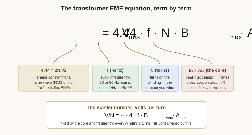
That question has a surprisingly orderly answer. Transformer design is not guesswork and it is not, at the level a builder needs, advanced mathematics. It is a short chain of decisions, each feeding the next, anchored by a single equation that everything else hangs from — the electromotive-force equation, universally written

V(rms) = 4.44 · f · N · Bmax · Ac

Learn to read that equation both forwards and backwards and the whole design flow opens up. Forwards, it tells the volts a winding of N turns will produce on a given core; backwards, it tells the turns needed for a target voltage. Everything else in the flow — picking the core, choosing the flux, sizing the wire, checking that the copper fits and the thing stays cool — is engineering judgment layered around that one relationship. This volume walks the whole chain, term by term and then twice in full: once for a classic 50/60 Hz mains transformer wound on iron laminations, and once, in sketch, for a 100 kHz switch-mode flyback on a gapped ferrite core, so the reader sees how the same physics produces wildly different transformers when the frequency changes by four orders of magnitude.

The core materials and their frequency ranges were the subject of Volume 4, and the magnet wire, insulation classes, and safety creepage of Volume 5; this volume leans on both without re-deriving them. Regulation and efficiency — how much the output sags under load and how much power is lost as heat — were defined in Volume 2, and reappear here as budgets the design must meet. What is new is the act of synthesis: choosing all of those quantities together so that they are mutually consistent and the finished transformer meets its spec.

9.2 The design flow, at a glance

Before the arithmetic, it helps to see the whole route. A transformer design proceeds through eight steps, and the last of them can loop back to the start:

1. Write the specification. The required secondary voltage(s) and current(s), hence the volt-ampere (VA) rating; the supply voltage and frequency; the allowable regulation (voltage droop from no load to full load); and the allowable temperature rise. These are the givens.
2. Choose the core material and family. Frequency decides material: silicon steel for mains, ferrite for tens-to-hundreds of kilohertz, powdered iron or amorphous for special cases. The mechanical family (EI, toroid, C-core, shell) follows from cost, leakage, and how the thing will be wound.
3. Choose the working flux density Bmax. Below the material’s saturation flux Bsat, with margin, and low enough that core loss stays inside the temperature budget.
4. Size the core. The area-product method — Ap = Wa · Ac — turns the VA rating, frequency, flux, current density, and fill factor into a minimum core size, which is then matched to a real, catalogued core.
5. Find volts-per-turn, then turns. Volts-per-turn = 4.44 · f · Bmax · Ac is fixed by the chosen core and frequency; each winding’s turns is its voltage divided by that number, with a few percent added to the secondary for regulation.
6. Size the wire. Each winding’s current, divided by a chosen current density J, gives the copper cross-section, which rounds to a wire gauge.
7. Check the window fit. The total copper — every winding’s turns times its wire area — must fit inside the core window at a realistic fill factor Ku. If it does not, the core is too small.
8. Check losses, regulation, and temperature rise. Sum copper and core loss, compare the resistive drop against the regulation budget, and compare the heat against the surface area that must shed it. If any check fails, iterate: a bigger core, a lower flux, or a fatter wire, and around again.

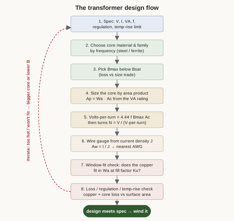
The loop in step 8 is the heart of real design. A first pass almost never lands perfectly; the copper is a hair too fat for the window, or the calculated temperature rise is ten degrees over budget, and the designer steps back to the core choice and tries the next size up. What follows treats each step in turn, then runs the whole loop end to end on two concrete examples.

9.3 The EMF equation, read term by term

Every number in a transformer design descends from Faraday’s law of induction, which says the voltage induced in a coil equals the rate of change of the magnetic flux linking it, times the number of turns: v = −N · dΦ/dt. Volume 6 worked this into the transformer’s steady-state form. In an AC transformer the flux is (ideally) sinusoidal, Φ(t) = Φmax · sin(2πf t), so its rate of change is a cosine of peak amplitude 2πf · Φmax. The induced voltage is therefore also sinusoidal, with a peak of 2πf · N · Φmax. Meters and specifications deal in root-mean-square (RMS) volts, not peaks, and for a sine wave RMS = peak / √2. Dividing the peak by √2 gives

V(rms) = (2π / √2) · f · N · Φmax = 4.44 · f · N · Φmax

The famous constant 4.44 is nothing more mysterious than 2π/√2 = 6.2832 / 1.4142 = 4.4429. It is a sine-wave shape factor; it appears because the supply is a sinusoid. Drive the same core with a square wave, as a switch-mode converter does, and the shape factor becomes 4.0 instead, a point the flyback example will use.

The peak flux Φmax, in webers, is just the peak flux density Bmax (in tesla) multiplied by the cross-sectional area of the core Ac (in square metres): Φmax = Bmax · Ac. Substituting gives the equation in the form every design uses:

V(rms) = 4.44 · f · N · Bmax · Ac

Read it as a sentence: the RMS volts on a winding equal a sine-wave constant, times how fast the field alternates, times how many turns catch it, times how much iron the field passes through, times how hard the iron is driven. Each term is a lever a designer can pull. Two of them — Bmax and Ac — belong to the core and are chosen once; two of them — V and N — belong to the winding and trade against each other; one — f — is set by the supply and is usually a given.

Rearranging isolates the single most useful quantity in transformer work, volts per turn:

V / N = 4.44 · f · Bmax · Ac

Once the core (Ac), the material (which caps Bmax), and the frequency (f) are fixed, volts-per-turn is a single fixed number for the whole transformer, shared by every winding on that core. This is the master number. Every winding’s turn count is simply its required voltage divided by volts-per-turn. A design becomes a bookkeeping exercise: compute one number, then divide each voltage by it.

9.3.1 Why AC only, restated as a design fact

The equation quietly re-explains why a transformer cannot run on DC. If f = 0, then volts-per-turn = 0: no changing flux, no induced voltage, no matter how many turns are wound. Worse, a DC voltage across a winding is limited only by its (tiny) copper resistance, so the current climbs until the core saturates and the winding cooks. The frequency term is not a formality; it is the whole mechanism.

9.4 Choosing the core: material, then flux, then size

9.4.1 Material by frequency

Volume 4 laid out the materials in detail; design only needs their headline consequences. Grain-oriented (GO) silicon steel — thin laminations, saturation around 1.9–2.0 T — is the material of mains transformers because its core loss is acceptable at 50/60 Hz and it packs a lot of flux into a small area. Push it to tens of kilohertz and its eddy-current loss becomes ruinous no matter how thin the laminations, which is why switch-mode converters abandon steel for ferrite — a ceramic magnetic material with saturation only around 0.3–0.5 T but with loss low enough to run at hundreds of kilohertz. Powdered iron, amorphous, and nanocrystalline cores fill the niches between. The single rule the designer carries forward: let the frequency choose the material, then work within that material’s flux ceiling.

9.4.2 Flux density: below saturation, with margin

The choice of Bmax is a trade, and a consequential one. The EMF equation rewards a high Bmax — the higher the flux, the more volts each turn makes, so the fewer turns and the smaller the core. But two penalties climb with flux. First, core loss (hysteresis plus eddy) rises steeply with Bmax; the classic Steinmetz relation makes hysteresis loss climb faster than linearly, so a core run near saturation runs hot. Second, and more dangerous, is saturation on transients. Mains voltage can surge; the flux at switch-on can momentarily double (the inrush of Volume 2). A core designed to sit at 1.8 T at nominal voltage will be slammed hard into saturation by any over-voltage or by the DC offset of a half-cycle inrush, drawing enormous current.

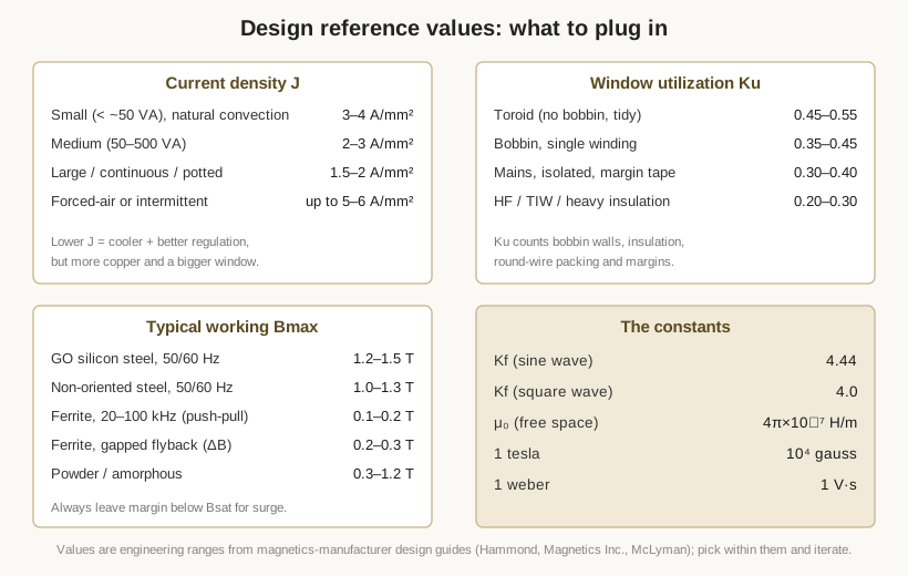
The working compromise for GO steel at 50/60 Hz is Bmax around 1.2–1.5 T — comfortably below the ~1.9 T saturation, leaving headroom for surge and keeping core loss moderate. Ferrite in a push-pull converter runs at 0.1–0.2 T (loss, not saturation, is the limit at high frequency), and a gapped flyback swings ΔB of 0.2–0.3 T. The worked examples use 1.2 T for the mains design and 0.25 T for the flyback, both deliberately conservative.

9.4.3 Sizing the core: the area-product method

The equation says nothing directly about how big a core a given VA rating needs. Two independent constraints set the size, and the area-product method combines them.

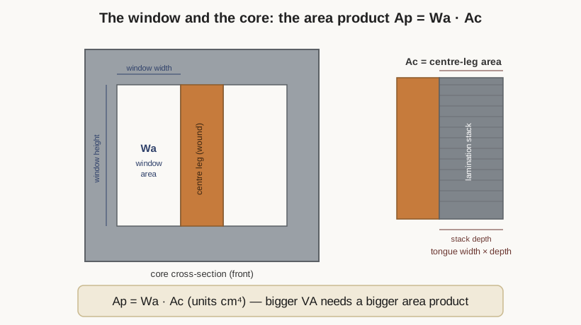
The core cross-section Ac sets volts-per-turn, and hence the total number of turns for a given voltage. The core window area Wa — the open space between the legs, where the wire goes — sets how much copper can be packed in, and hence how much current the windings can carry. A transformer needs both enough Ac to make its volts at a sane turn count and enough Wa to fit the copper for its amps. The product of the two,

Ap = Wa · Ac

(the area product, in units of length⁴, usually cm⁴), is the single figure of merit that scales with power-handling. Manufacturers publish it, often disguised as a VA rating for a stated frequency and temperature rise.

The area product needed for a given design follows from the EMF equation and the wire sizing, combined. Derived in the standard references (McLyman’s handbook is the canonical one), the relation is, in SI units with Ap in m⁴,

Ap = Pt / (Kf · f · Bmax · J · Ku)

where Pt is the total apparent power the windings handle (in volt-amperes — for a two-winding transformer, roughly the sum of the primary and secondary VA, near 2× the output VA), Kf is the shape factor (4.44 sine, 4.0 square), J is the current density in A/m², and Ku is the window utilization factor (the fraction of the window that ends up as bare copper). The same relation, with Ap in cm⁴, Bmax in tesla, f in hertz, and J in the practical unit of amps per cm², carries a factor of 10⁴:

Ap (cm⁴) = Pt · 10⁴ / (Kf · f · Bmax · J · Ku)

Read the numerator and denominator as levers. More power (Pt) needs a bigger core. Higher frequency, flux, current density, or fill all shrink the core needed — which is exactly why a 100 kHz ferrite transformer of the same VA is a fraction of the size of a 60 Hz iron one: the f in the denominator is more than a thousand times larger. The method’s job is core selection: compute the required Ap, then pick the smallest catalogued core whose published Ap meets or exceeds it. The worked mains example below does this both ways — computing turns and wire first, then confirming the area product comes out consistent.

9.5 Turns, wire, and the window fit

9.5.1 Turns from volts-per-turn

With the core (Ac), material (Bmax), and frequency (f) fixed, volts-per-turn is a single number and each winding’s turns is a division:

N = V / (4.44 · f · Bmax · Ac)

The primary uses the supply voltage directly. Each secondary uses its target output voltage — but with a wrinkle. Under load, the secondary’s own winding resistance drops some voltage, so a secondary wound for exactly its rated turns will read low at full load. The fix is to add turns to the secondary to pre-compensate — typically a few percent, matched to the regulation the design is targeting. A 5% regulation transformer gets roughly 5% extra secondary turns; a stiff, well-regulated one gets more. The primary is not padded this way, because the primary sets the flux and adding primary turns lowers volts-per-turn for everything.

The single-number nature of volts-per-turn is what makes multiple outputs and taps trivial to design. A transformer with a 24 V and a 12 V secondary is not two designs; it is 122 turns for one and 61 for the other on the same 0.208 V/turn core, each padded for its own regulation. A centre-tapped secondary is simply a tap brought out at the halfway turn. A multi-tap mains primary for 120/230 V operation is the same trick on the input side: turns counted to give the right flux at each tapping voltage. Because they all share one volts-per-turn, the windings interleave and stack on the same bobbin, and the only new bookkeeping is the current each carries, which feeds its own wire-gauge and window-fit line in the sum.

9.5.2 Wire from current density

The wire gauge follows from how much current each winding carries and how hard the copper may be worked. Current density J, in amps per square millimetre, is the knob. Run the copper hard (high J) and the wire is thin, the winding small and cheap, but resistive and hot; run it soft (low J) and the winding is fat, cool, and well-regulated but bulky. For small transformers cooled by natural convection the customary range is 2–4 A/mm², dropping to 1.5–2 A/mm² for large or continuously-loaded units and rising to 5–6 A/mm² where forced air or intermittent duty allows. The required bare-copper cross-section for a winding carrying current I is simply

Aw = I / J

which is then rounded up to the next standard wire gauge. (The American Wire Gauge table and its per-gauge copper areas were given in the Coils dive and in this dive’s Volume 5; a fistful of anchor points: AWG 26 ≈ 0.128 mm², AWG 22 ≈ 0.326 mm², AWG 19 ≈ 0.653 mm², AWG 16 ≈ 1.31 mm², each step of three gauges roughly doubling area.)

9.5.3 The window utilization factor and the fit check

Not all of the window becomes copper. The bobbin walls take space, the interlayer and barrier insulation take space, round wire cannot tile a plane without gaps, and mains designs waste the margin strips at each end of every layer for creepage. The fraction of the raw window Wa that actually ends up as bare copper is the window utilization factor Ku, and it is stubbornly less than one. Typical values: 0.4–0.5 for a tidy toroid or a simple single-winding bobbin; 0.3–0.4 for a mains transformer with isolation and margin tape; 0.2–0.3 for a high-frequency winding built with triple-insulated wire and heavy interlayer film. A common all-purpose default for mains work is Ku = 0.4.

The fit check is then a single inequality. Add up the bare copper of every winding — for each, its turns times its wire’s copper area — and require that it fit inside the window at the chosen Ku:

Σ (N · Aw) ≤ Wa · Ku

If the copper does not fit, the design has run out of window and the remedy is a bigger core (more Wa), a higher current density (thinner wire, hotter), or a higher flux (fewer turns) — the iterate loop. If it fits with room to spare, the core may be larger than it needs to be, and a smaller one can be tried to save cost and weight.

9.6 Regulation, losses, and temperature rise as budgets

Steps 5 through 7 produce a transformer that works electrically. Step 8 asks whether it works thermally and within its regulation budget — and these three quantities are the ones that most often send a design back around the loop.

Copper loss is the I²R heating in the windings, and it is set by the wire sizing: thinner wire (higher J) means more resistance and more loss. It rises and falls with load. Core loss is the hysteresis-plus-eddy heating in the iron, set by the flux and frequency; it is roughly constant with load (it depends on the flux, which the supply voltage fixes) and is the dominant loss at light load. Volume 2 treated both in detail. The design uses them two ways.

First, regulation. The full-load copper loss, expressed as a voltage drop across the winding resistances, is the bulk of the voltage droop from no load to full load. If the spec allows 5% regulation and the computed resistive drop is 8%, the wire is too thin — drop J and refatten it, or add still more secondary turns.

Second, temperature rise, which is where losses meet geometry. All of the loss — copper plus core — becomes heat, and that heat must leave through the transformer’s surface area. A small transformer has little surface relative to its volume, so a given number of watts raises its temperature more. The rough engineering rule ties total loss to surface area through a surface heat-transfer coefficient; a natural-convection transformer sheds very roughly on the order of a few hundred milliwatts per square centimetre of surface for a 40–50 °C rise. If the summed loss divided by the available surface predicts a rise past the insulation-class limit (the thermal classes of Volume 5 — Class A at 105 °C, Class B at 130 °C, and so on), the design is thermally illegal and must grow: a bigger core has both more surface and room for fatter, cooler wire. This is the deepest reason the area-product method works — a core sized for a given VA at a stated temperature rise has, built into its published rating, enough surface to shed the losses that VA implies.

9.7 Worked design 1: a 120 V, 60 Hz to 24 V, 2 A mains transformer

Now the whole loop, end to end, on a classic linear-supply transformer. The specification: a 48 VA transformer, primary 120 V at 60 Hz, secondary 24 V at 2 A, natural convection, modest regulation. Every number below is shown.

Step 1 — spec. Output VA = 24 V × 2 A = 48 VA. Primary current, ignoring losses for a first pass, ≈ 48 VA / 120 V = 0.4 A. Supply 120 V, 60 Hz.

Step 2 — material and family. Sixty hertz means silicon-steel laminations; an EI core is the classic, cheap, easily-wound choice. Choose a core with a centre-leg cross-section Ac = 6.5 cm² = 6.5 × 10⁻⁴ m² (a common mid-size EI stack, e.g. a 1.5-inch tongue with a matching stack height).

Step 3 — flux. GO steel saturates near 1.9 T; work at Bmax = 1.2 T for margin and moderate core loss.

Step 5 — volts-per-turn (taking core size as given from a catalogue for now, and confirming the area product at the end):

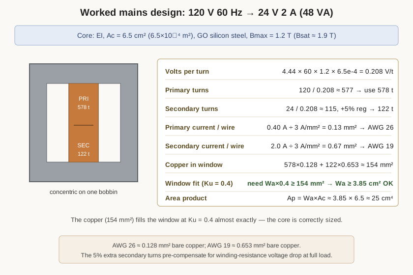
V/N = 4.44 × f × Bmax × Ac = 4.44 × 60 × 1.2 × 6.5×10⁻⁴

Working it: 4.44 × 60 = 266.4; × 1.2 = 319.68; × 6.5×10⁻⁴ = 0.2079 V per turn. About a fifth of a volt per turn — a typical figure for a small mains transformer.

Turns.

• Primary: N₁ = 120 / 0.2079 = 577.2 → round to 578 turns.
• Secondary, base: N₂ = 24 / 0.2079 = 115.4 turns. Add ~5% for regulation: 115.4 × 1.05 = 121.2 → 122 turns.

Step 6 — wire. Current density J = 3 A/mm² (small, natural convection).

• Secondary: Aw = 2.0 A / 3 = 0.667 mm². Diameter √(4 × 0.667 / π) = 0.92 mm; the nearest standard is AWG 19 (0.912 mm, 0.653 mm² bare copper).
• Primary: Aw = 0.40 A / 3 = 0.133 mm². Diameter 0.41 mm; nearest is AWG 26 (0.405 mm, 0.128 mm² bare copper).

Step 7 — window fit. Total bare copper:

N₁ × Aw₁ + N₂ × Aw₂ = 578 × 0.128 + 122 × 0.653 = 74.0 + 79.7 = 153.7 mm²

At Ku = 0.4, the raw window must be at least 153.7 / 0.4 = 384 mm² = 3.84 cm². An EI core with Ac = 6.5 cm² has a window comfortably larger than this (a typical such core offers roughly 4–5 cm²), so the copper fits.

Confirming the area product. With Wa ≈ 3.85 cm² and Ac = 6.5 cm², the area product is Ap = Wa × Ac ≈ 3.85 × 6.5 ≈ 25 cm⁴. The area-product formula predicts the same. Taking Pt ≈ 2 × 48 = 96 VA (primary VA plus secondary VA), Kf = 4.44, f = 60, Bmax = 1.2 T, J = 3 A/mm² = 300 A/cm², Ku = 0.4:

Ap = Pt × 10⁴ / (Kf × f × Bmax × J × Ku) = 96 × 10⁴ / (4.44 × 60 × 1.2 × 300 × 0.4)

Denominator: 4.44 × 60 = 266.4; × 1.2 = 319.68; × 300 = 95 904; × 0.4 = 38 362. Numerator 960 000. Ap = 960 000 / 38 362 = 25.0 cm⁴. The two routes agree — the core is correctly sized, neither starved nor wasteful.

Step 8 — checks. The winding resistances, from the wire lengths and gauges, set the copper loss and the regulation. Take a mean length per turn (MLT) — the average circumference of one turn around the bobbin — of roughly 12 cm for the inner primary and 14 cm for the outer secondary (both read off the core’s window and stack dimensions; the outer winding is longer because it sits over the primary). Then:

• Primary wire length ≈ 578 × 0.12 m = 69 m of AWG 26. AWG 26 copper is ≈ 0.134 Ω/m, so R₁ ≈ 69 × 0.134 ≈ 9.3 Ω. Primary copper loss = I²R = 0.4² × 9.3 ≈ 1.5 W.
• Secondary wire length ≈ 122 × 0.14 m = 17 m of AWG 19. AWG 19 copper is ≈ 0.0264 Ω/m, so R₂ ≈ 17 × 0.0264 ≈ 0.45 Ω. Secondary copper loss = 2² × 0.45 ≈ 1.8 W.

Total copper loss ≈ 3.3 W, plus a core loss of order 1 W for a ~1 kg GO stack at 1.2 T and 60 Hz — call it ~4.3 W total, an efficiency near 48 / (48 + 4.3) ≈ 92%, respectable for a 48 VA transformer. For regulation, the secondary’s own 0.45 Ω drops 2 A × 0.45 = 0.9 V (3.8% of 24 V), and the primary’s resistance, referred to the secondary, adds a few percent more — together on the order of 6–7% before compensation. The 5% of extra secondary turns wound in Step 5 cancels most of it, landing the loaded output close to 24 V. Finally, ~4.3 W spread over the perhaps 150–200 cm² of exposed surface of a core this size predicts a temperature rise well inside a Class-A (105 °C) insulation budget in open air. Every check passes, so no iteration is needed. The design is done: 578 turns of AWG 26 over 122 turns of AWG 19 on a 6.5 cm² EI core.

(These loss numbers depend on the assumed mean-length-per-turn and are representative, not exact — the true MLT is measured off the wound bobbin, and Volume 13 shows how the short-circuit test recovers the real copper loss and the open-circuit test the real core loss from the finished transformer.)

That is a complete, buildable mains transformer, arrived at with nothing more exotic than one equation and a table of wire gauges.

9.8 Worked design 2: a 100 kHz flyback, in sketch

Change the frequency by four orders of magnitude and the same physics produces a transformer that looks nothing like the first. A flyback — the workhorse of small switch-mode supplies (phone chargers, standby rails) — is a special beast: it stores energy in the gap of its core during the switch’s on-time and dumps it to the secondary during the off-time, so it is as much a coupled inductor as a transformer. But the turns still come from a volt-second balance descended from the same EMF idea, and seeing the numbers side by side with the mains design is the point.

Spec. Rectified-mains DC input, take Vin = 120 V (dc bus, minimum); switching frequency f = 100 kHz; maximum duty cycle Dmax = 0.45; output roughly 24 W. Core: a small gapped ferrite (EE or RM class) with Ac = 0.6 cm² = 0.6 × 10⁻⁴ m². Because the flux swings one way only (unidirectional), the usable swing is a ΔB of 0.25 T — a fifth of the mains design’s flux, because ferrite’s loss ceiling and saturation are both low.

Primary turns from the volt-second balance. During the on-time the input voltage is impressed across the primary and the flux ramps; requiring the flux swing to equal ΔB over the on-time gives the flyback’s turns equation:

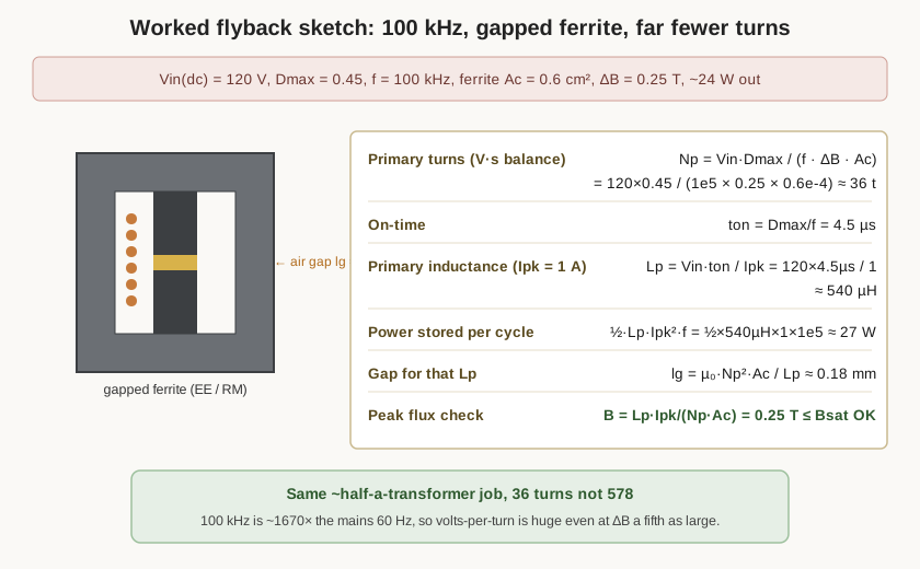
Np = Vin × Dmax / (f × ΔB × Ac) = 120 × 0.45 / (100 000 × 0.25 × 0.6×10⁻⁴)

Numerator: 120 × 0.45 = 54. Denominator: 100 000 × 0.25 = 25 000; × 0.6×10⁻⁴ = 1.5. Np = 54 / 1.5 = 36 turns. Set against the mains design’s 578, the contrast is the whole lesson: at 1670 times the frequency, even with a fifth of the flux and a tenth of the core area, the primary needs sixteen times fewer turns. The frequency term in the denominator dominates everything.

Primary inductance and peak current. A flyback’s primary is sized to store the right energy per cycle. The current ramps linearly during the on-time ton = Dmax / f = 0.45 / 100 000 = 4.5 µs, reaching a peak Ipk. Choosing Ipk = 1.0 A as the design peak, the primary inductance that produces that ramp is

Lp = Vin × ton / Ipk = 120 × 4.5×10⁻⁶ / 1.0 = 540 µH

The energy delivered per cycle confirms the power: ½ × Lp × Ipk² × f = 0.5 × 540×10⁻⁶ × 1² × 100 000 = 27 W of stored-and-transferred power, which at ~90% efficiency gives the ~24 W output targeted.

The gap. Ferrite’s permeability is so high that 36 ungapped turns would give far more than 540 µH and would saturate instantly; the inductance is set by a deliberate air gap. From Lp = μ₀ · Np² · Ac / lg, the gap length is

lg = μ₀ × Np² × Ac / Lp = (4π×10⁻⁷) × 36² × 0.6×10⁻⁴ / 540×10⁻⁶

Numerator: 4π×10⁻⁷ = 1.257×10⁻⁶; × 1296 = 1.629×10⁻³; × 0.6×10⁻⁴ = 9.77×10⁻⁸. Divide by 540×10⁻⁶: lg = 1.8×10⁻⁴ m = 0.18 mm — a gap ground into the centre leg, or set with a shim, of under two-tenths of a millimetre.

Saturation check. The peak flux density is B = Lp × Ipk / (Np × Ac) = 540×10⁻⁶ × 1.0 / (36 × 0.6×10⁻⁴) = 540×10⁻⁶ / 2.16×10⁻³ = 0.25 T, exactly the ΔB assumed, and safely under ferrite’s ~0.35–0.4 T saturation. Self-consistent.

The secondary follows from the reflected-voltage relationship rather than a simple volts-per-turn division: for a chosen reflected voltage of, say, 100 V, the primary-to- secondary turns ratio is 100 / (Vout + diode drop), so a 12 V output with a 0.7 V rectifier needs Np/Ns ≈ 100 / 12.7 ≈ 7.9, hence Ns ≈ 36 / 7.9 ≈ 5 turns. Five turns for the secondary, thirty-six for the primary — a whole switch-mode transformer wound in the turn count a mains transformer spends on a single tap.

The flyback design has more to it than this sketch — RMS currents for wire sizing, proximity-effect losses that push toward Litz or foil, snubbers, the exact reflected voltage that trades primary against secondary stress — and those belong to a dedicated SMPS treatment. But the skeleton is the same skeleton as the mains design: pick a core and a flux, get the primary turns from the frequency and area, size everything to fit, and check that nothing saturates or overheats.

9.9 What the two designs teach together

Set the two side by side and the design engine stands out clearly.

Table 1 — What the two designs teach together

Quantity	Mains (linear supply)	Flyback (SMPS)
Frequency f	60 Hz	100 kHz
Core material	GO silicon steel	gapped ferrite
Core area Ac	6.5 cm²	0.6 cm²
Working flux	Bmax = 1.2 T	ΔB = 0.25 T
Shape factor	4.44 (sine)	volt-second balance
Primary turns	578	36
Secondary turns	122	~5
Air gap	none	~0.18 mm

Every difference in the right-hand column traces back to that one factor of ~1670 in frequency. High frequency makes volts-per-turn enormous, which collapses the turn count, which shrinks the copper, which shrinks the core — the reason a modern phone charger the size of a matchbox does what a brick-sized linear transformer once did. The penalty, paid in the material and in the loss physics of Volume 4, is that ferrite’s low flux and the need for a precise gap make the high-frequency design fussier; but the method — the eight-step loop — is identical.

9.10 Handing off to the bench

A design on paper is a turns count, a pair of wire gauges, and a core part number. Making it real is the subject of the next three volumes. Volume 10 covers the winding machines — the coil winders that lay the 578 turns of AWG 26 down evenly, the traverse that spaces them across the bobbin, the turns counter that stops at exactly 578, and the tensioner that keeps the wire taut without stretching it. Volume 11 is the hands-on craft: preparing the bobbin, winding the primary, laying interleaving insulation between primary and secondary, bringing out taps and leads, stacking and interleaving the EI laminations, and impregnating the finished coil with varnish. Volume 12 takes the designs to worked builds, including a mains transformer close to the 48 VA example above.

Two threads close the loop back to this volume. The regulation and temperature-rise budgets sketched here are verified on the finished transformer in Volume 13, where the open-circuit and short-circuit tests measure the very core and copper losses the design estimated. And the equations, constants, and design tables used throughout are collected as a one-page cheat sheet in Volume 14 — the EMF equation, the area-product formula, the current-density and Ku ranges, and the wire tables — so the whole eight-step flow can be run at the bench from a single reference card.

The transformer that seemed, in Volume 1, like an almost magical black box that turns one voltage into another is now, at the end of the design engine, entirely demystified: it is 4.44 · f · N · Bmax · Ac, solved for the turns, wound in wire thick enough to carry the current and thin enough to fit the window, on a core big enough to make the volts and shed the heat. Everything else is craft — and the craft is where the dive goes next.