Types II: Instrument, RF, and Switch-Mode Transformers

8.1 The other half of the family

The previous volume walked the transformers that live on the mains and in the audio path — power and isolation transformers, autotransformers and variacs, the tube output transformer and its impedance-matching cousins. Those are the transformers a person meets as objects: heavy iron things that hum, or the tidy toroid inside an amplifier. This volume covers the rest of the family, and it is a stranger, more specialised set. These transformers are less often admired for their own sake because they hide inside instruments, radios, antenna feed points, and the ticking guts of every switching power supply on the planet. Yet between them they outnumber every mains transformer ever wound, and three of the four classes here break the comfortable picture of “iron core, 50 or 60 hertz, volts in and volts out” in an instructive way.

The four classes are instrument transformers, which do not deliver power at all but manufacture a small, safe, faithful replica of a large and dangerous current or voltage so that a meter or a protection relay can look at it; radio-frequency transformers, which work up where the wavelength shrinks to metres and the core stops being iron and becomes ferrite or nothing at all; baluns and ununs, a family of transmission-line transformers that transform impedance by a trick of wave propagation rather than by flux linkage, and are broadband because of it; and switch-mode transformers, the ferrite hearts of modern power conversion, one of which — the flyback — is not really a transformer at all but an energy-storing coupled inductor wearing a transformer’s clothes.

Each is treated the same way: what it is, how it is built, what it is for, and where its trade-offs bite. Two threads run underneath. The first is that core material and operating frequency are joined at the hip, a point made in Volume 4 (core materials) and Volume 6 (transformer action) and paid off here: as frequency climbs from the mains through the audio band into the megahertz and beyond, the core shrinks, changes chemistry from silicon steel to ferrite, and eventually vanishes. The second is that the humble turns ratio of Volume 1 keeps reappearing in disguise — as a current ratio in the CT, as an impedance ratio in the balun, as the storage-and-release ratio of the flyback — so that a reader who has the ampere-turn balance and the N² impedance law firmly in hand will find nothing here truly foreign.

8.2 Instrument transformers: measuring what you dare not touch

An instrument transformer exists to let a small, cheap, grounded instrument measure a quantity that is too large, too high in voltage, or too hazardous to connect to directly. A panel ammeter cannot carry the 800 amps flowing in a switchboard busbar; a metering-grade voltmeter cannot be wired across an 11 000 volt line and survive, still less be touched by the person reading it. The instrument transformer sits between the dangerous circuit and the safe one and provides a scaled, isolated copy. There are two kinds: the current transformer (CT), which produces a small secondary current proportional to a large primary current, and the voltage or potential transformer (VT / PT), which produces a small secondary voltage proportional to a large primary voltage.

8.2.1 The current transformer

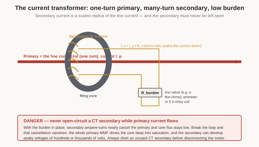
A current transformer inverts the everyday intuition about what a “primary” is. On a mains transformer the primary is an obvious winding of many turns. On a CT the primary is often a single turn — frequently just the main conductor itself, the fat busbar or cable, passed once through the middle of a ring core. The secondary is a many-turn winding on that ring, brought out to a pair of terminals. Because the ampere-turn balance of Volume 6 still holds — primary ampere-turns must be matched by secondary ampere-turns — a large primary current in one turn is reproduced as a small secondary current in many turns, scaled down by the turns ratio. A CT wound with 200 secondary turns, with the busbar as its one-turn primary, turns 1000 amps in the bar into 5 amps at the terminals: a ratio of 200:1, conventionally written 1000:5. The near-universal secondary rating is 5 amps (1 amp is common in high-burden installations), because switchboard meters and relays were standardised around that figure a century ago.

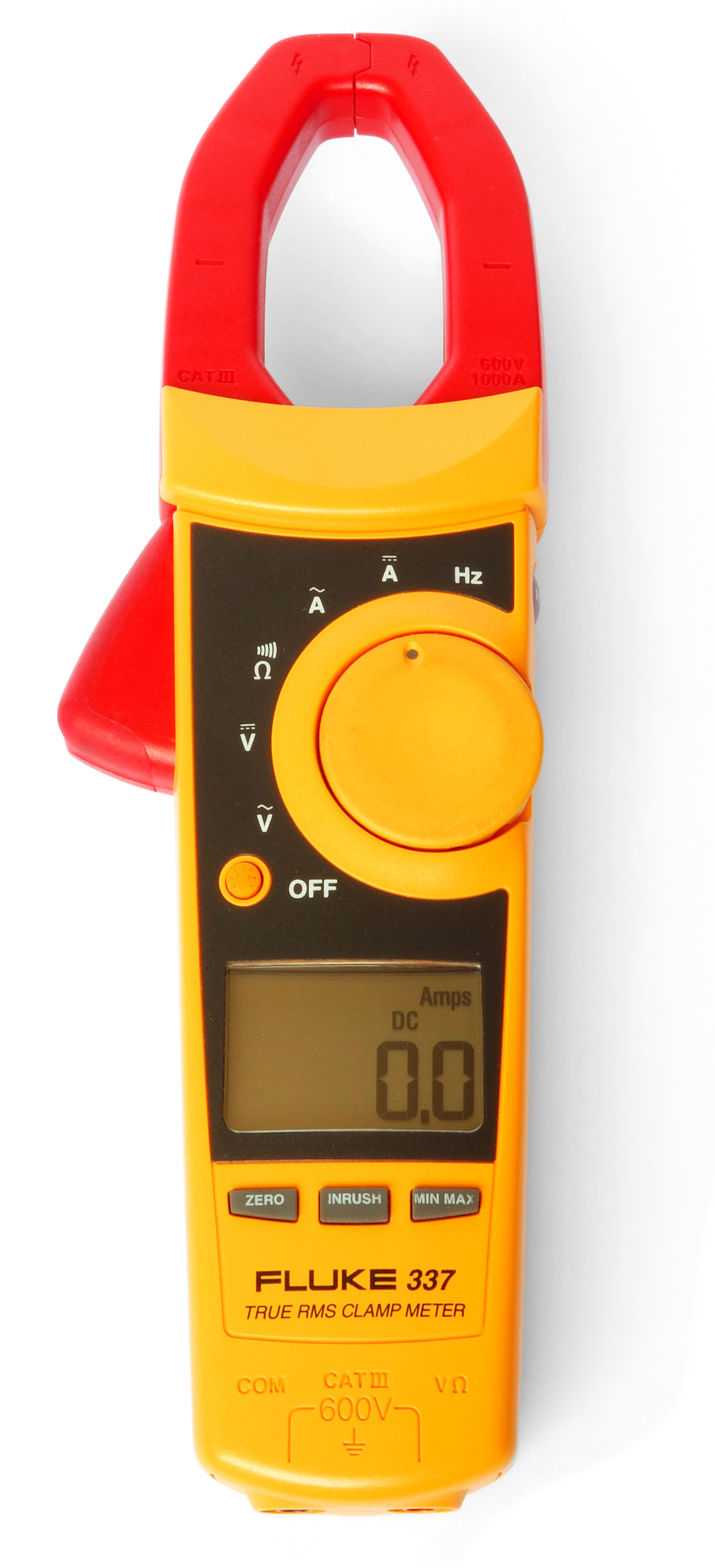
The most familiar CT in the world is the one inside a clamp meter (Figure 1). Its hinged jaws are a ferrite or silicon-steel core split across one face; opening the jaws parts the core, closing them around a wire re-forms a complete magnetic ring with that wire threaded through it as a one-turn primary. The secondary is a fixed multi-turn winding buried in the jaw assembly. Nothing has to be disconnected — the beauty of the CT is that it senses current without breaking into the circuit — and the instrument reads the scaled-down secondary current (or, in an AC/DC clamp, uses a Hall sensor for the DC part, which is a different story). The same principle, made permanent, is the switchboard CT: a toroid factory-wound with its secondary, slipped over a busbar during construction.

The load on a CT’s secondary has a special name: the burden. It is deliberately kept low — a few ohms, the resistance of the ammeter coil or the protection relay plus the wiring — and it is specified not in ohms but in volt-amperes at rated secondary current, because that is what determines how hard the core has to work. A “15 VA” CT can drive 15 VA of meters and leads at 5 amps (that is, up to 0.6 ohm) while holding its rated accuracy. Push more burden than that on it and the secondary voltage needed to force the rated current through the load climbs, the core has to sustain more flux, and the ratio error grows as the magnetising branch (Volume 2) steals a larger fraction of the primary ampere-turns. Under-burden a CT and accuracy also suffers slightly; the IEC standard for instrument transformers, IEC 61869, quotes CT accuracy for burdens between about a quarter and the full rated VA.

CTs come in a few physical forms that all obey the same electrical rules. A window or ring CT is the bare toroid described above: the conductor is threaded through the hole, so the user supplies the one-turn primary. A bar or bushing CT has a solid bar built in as its one-turn primary and is bolted into the busbar run; the large donut CTs that ride on transformer bushings in a substation are of this kind. A wound-primary CT, used at lower currents where one turn would give too little signal, has an actual multi-turn primary winding — this is the form of a small panel or PCB-mount current-sense transformer that reads, say, 20 amps by winding several primary turns to lift the ampere-turns to a usable level. In every case the governing quantity is the primary ampere-turns (current times primary turns), which is why threading the sensed wire through a window CT twice halves its effective ratio: two primary turns double the ampere-turns for the same current.

8.2.2 Metering cores versus protection cores

A CT core is asked to do one of two opposite jobs, and a good design cannot do both at once. A metering CT must be accurate around normal load current so that the energy meter or panel ammeter reads true; its accuracy classes are labelled by their worst-case ratio error, 0.1, 0.2, 0.5, 1 (and the “s” variants 0.2S, 0.5S that hold accuracy down to very light loads). A class 0.5 metering CT keeps its ratio error inside ±0.5 % from roughly 5 % to 120 % of rated current. Crucially, a good metering CT is designed to saturate soon above its normal range: if a fault sends twenty times rated current down the line, the last thing anyone wants is for that surge to be faithfully reproduced into a delicate 5-amp meter movement, so the core rolls off and protects the instrument.

A protection CT wants the exact reverse. During a fault it must keep reproducing the current faithfully, well past rated, so that the protection relay sees a true picture of the fault and trips correctly. Its class is written like 5P10 or 5P20: the number after the P is the accuracy limit factor, the multiple of rated current up to which the composite error stays within the stated percentage. A 5P20 core holds its error inside 5 % all the way to twenty times rated current — it is built with enough core cross-section to avoid saturating on a heavy fault. Because metering and protection make opposite demands on the iron, serious switchgear often carries two separate CT cores on the same busbar, one tuned for the meter and one for the relay, each with its own secondary winding.

8.2.3 The one rule that can kill you: never open the secondary

Every safety briefing about current transformers reduces to a single imperative, and it is worth understanding rather than merely obeying. In normal operation the secondary current flows through its low burden, and those secondary ampere-turns sit almost exactly opposite the primary ampere-turns. The two nearly cancel, the net magnetomotive force on the core is tiny, and the core flux — and therefore the secondary voltage — stays modest. This is why a CT can have a one-turn primary and still behave: the burden is what holds the whole thing in check.

Now open the secondary while primary current still flows in the busbar. The cancelling ampere-turns vanish in an instant. The full primary magnetomotive force is suddenly applied to the core with nothing to oppose it, and it drives the core hard into saturation on every half cycle. Each time the flux slams from one saturation extreme to the other, it does so through a near-vertical dB/dt, and the many-turn secondary — now effectively open — develops enormous voltage spikes across its terminals: hundreds of volts on a small CT, several kilovolts on a large one, enough to break down the winding insulation, destroy the CT, and electrocute anyone touching the terminals (Figure 2). The rule follows directly: a CT secondary must never be open-circuited while primary current flows. Before disconnecting a meter from a live CT, one first fits a shorting link across the secondary terminals. A shorted CT secondary is perfectly happy — it simply reads zero volts and the ampere-turns still cancel — whereas an open one is a bomb.

It is worth naming the modern alternative that sidesteps the open-secondary hazard entirely: the Rogowski coil. This is a toroidal winding on a flexible, air-cored (non-magnetic) former, clipped around the conductor like a CT. Having no iron to saturate, its output is not a scaled current but a voltage proportional to the rate of change of the primary current, which an integrator turns back into a current reading. Because there is no core, a Rogowski coil cannot saturate, is inherently safe when open-circuited, and handles enormous currents linearly — the trade being that it needs the active integrator and cannot read DC. It is not a transformer in the sense of this dive, but it competes directly with the protection CT and is worth recognising for what it is: a current sensor without the CT’s iron and without the CT’s lethal failure mode.

8.2.4 The voltage or potential transformer

Its counterpart, the voltage transformer (also potential transformer), is closer to an ordinary transformer in construction but is optimised for accuracy of ratio and phase rather than for delivering power. Its job is to step a high line voltage down to a standardised 110 volts (or 100 or 120, by region) that a metering voltmeter, wattmeter, or protection relay can safely handle. An 11 000-volt VT with a 100:1 ratio presents 110 volts to the instruments while isolating them — and the operator — from the line. Because a VT’s whole purpose is faithful ratio, it is run near open-circuit with only the light burden of instrument coils, and its accuracy classes (again 0.1, 0.2, 0.5, 1 under IEC 61869) constrain both magnitude error and phase-angle error, since a wattmeter or a directional relay depends on the phase being reproduced as truthfully as the amplitude. A VT is essentially a small, precise, lightly loaded step-down transformer whose regulation and phase shift have been engineered down to fractions of a percent. Between them the CT and the VT let a protection and metering panel that runs entirely on 5 amps and 110 volts supervise a substation carrying thousands of amps at tens of kilovolts — never touching either.

8.3 Radio-frequency transformers: coupling where the wavelength shrinks

Climb the frequency axis from the mains, through audio, and up past a few hundred kilohertz, and the transformer changes character. Silicon-steel laminations, with their eddy losses rising as the square of frequency, become useless; the core turns to ferrite — a ceramic of iron oxide with manganese-zinc or nickel-zinc — or, at the very top, disappears entirely into an air-cored coil. Two broad kinds of RF transformer matter here: the tuned transformer, which is deliberately part of a resonant circuit and therefore frequency-selective, and the broadband ferrite transformer, which is engineered to be as flat as possible across many octaves.

8.3.1 The tuned IF transformer

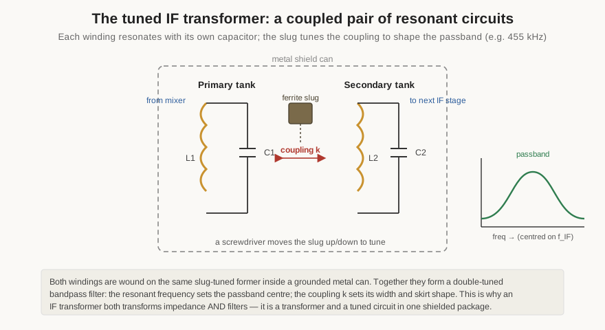
For much of the twentieth century the beating heart of every superheterodyne radio and television set was a little aluminium can, perhaps a centimetre square, with a screwdriver slot in the top: the intermediate-frequency (IF) transformer (Figure 3). Inside the can are two windings on a common former, plus one or two small capacitors, and a threaded ferrite slug (the “slug” or core) that can be screwed up and down inside the former. This is not merely a transformer; it is a transformer whose windings are each resonated with a capacitor, so that the whole assembly is a double-tuned bandpass filter as well as an impedance-matching link between one amplifier stage and the next.

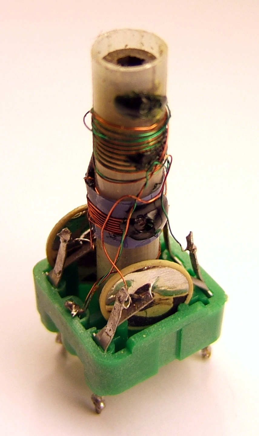
The superheterodyne receiver works by shifting every incoming station down to one fixed intermediate frequency — classically 455 kHz for AM broadcast radio, 10.7 MHz for FM, and 38–45 MHz for television — so that the fussy business of selectivity and gain can be done once, at that one frequency, by a chain of identical tuned stages. Each stage is coupled to the next by an IF transformer. Adjusting its slug moves the ferrite deeper into the coils, raising their inductance and lowering the resonant frequency; a technician “aligns” a receiver by tweaking every can in turn until the whole IF chain is centred on 455 kHz with the right bandwidth. The coupling between the two windings — set at manufacture and sometimes trimmed — controls the shape of the passband: loose coupling gives a narrow, peaked response, tighter coupling a wider, flatter, double-humped one (Figure 4). The metal can is not decoration; it is a shield that stops the high- impedance tuned circuit inside from radiating into, or picking up from, its neighbours, which would cause the whole cascade to oscillate.

The trade-off of the tuned transformer is exactly its selectivity: it works only in a narrow band around its resonance, and it must be tuned. That is a feature in a radio and a nuisance everywhere else, which is why the second kind of RF transformer exists.

8.3.2 Broadband ferrite RF transformers and impedance matching

Many radio jobs need the opposite of selectivity — a transformer that couples signal and transforms impedance uniformly across a huge frequency span: the input and output of a wideband amplifier, the port of a mixer, the primary of an antenna feed. These are broadband RF transformers, and they are wound on small ferrite toroids or two-hole binocular cores, usually of nickel-zinc ferrite, which has lower permeability but far lower loss at high frequency than the manganese-zinc grades used for power. A few turns of wire on such a core give an inductance whose reactance is already large compared with the circuit impedances by the bottom of the band, so the windings behave as an ideal transformer from there upward; the N² impedance law of Volume 1 does the rest. A common part is the surface-mount RF transformer that matches a 50-ohm line to some other impedance — 50:75, 50:200, or a 1:1 isolation unit used simply to break a ground loop or convert single-ended to differential. Because the whole point is flatness, these transformers are characterised by their insertion loss and return loss across a band (say 0.5 to 500 MHz) rather than by a turns ratio alone. A close relative is the centre-tapped RF transformer used to drive a push-pull mixer or amplifier: one winding split into two equal halves feeds two devices in antiphase, and the same part run backwards recombines their outputs. Catalogue houses such as Mini-Circuits and Coilcraft sell hundreds of these as sealed surface-mount parts specified by turns ratio, impedance ratio, bandwidth, and insertion loss rather than by any winding detail — a reminder that at RF the transformer has become a characterised black box. When the required bandwidth is truly enormous, though, even a few turns of ordinary flux-coupled winding run out of steam at the top, and the design crosses over into the transmission-line transformer — the balun.

8.4 Baluns and ununs: the transmission-line transformer

Two words that sound like jargon are worth unpacking, because they name the job precisely. A balun connects a balanced circuit to an unbalanced one. A balanced line — a dipole antenna’s two arms, an open-wire feeder, a differential amplifier’s two inputs — carries its signal as equal and opposite voltages on two conductors, neither of which is grounded. An unbalanced line — coaxial cable, a transmitter’s single-ended output — carries its signal on one conductor referenced to a grounded shield. Connect one directly to the other and the balance is broken: current that should have stayed inside the coax flows back along the outside of its shield, so the feedline radiates, distorts the antenna pattern, and brings RF back into the shack. A balun forces the two sides of the balanced circuit to carry equal and opposite currents while presenting an unbalanced face to the coax. An unun, by the same logic, joins an unbalanced circuit to another unbalanced one — no balance conversion, purely an impedance transformation — and is the device of choice at the base of an end-fed wire antenna.

8.4.1 Transformation by transmission line, not by flux alone

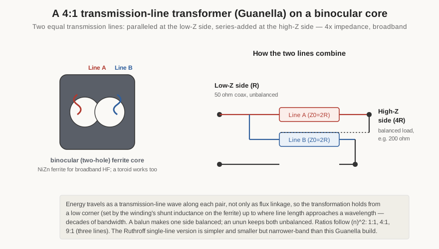
What makes baluns and ununs distinctive is how they transform impedance. An ordinary transformer relies wholly on flux linkage: the primary magnetises the core, the changing flux induces the secondary, and the ratio is set by turns. That works beautifully at one frequency but the leakage inductance and winding capacitance of a flux-coupled winding limit its high-frequency reach. A transmission-line transformer sidesteps the limit. Its windings are arranged as transmission lines — a bifilar pair, or a length of coax or twisted pair — wound onto a ferrite core, and the signal travels along them as a guided wave. The ferrite’s job is not to carry the main signal flux at all; it is to present a high impedance to any common-mode current (current flowing the same way on both conductors) so that the wanted differential wave passes freely while the unwanted common-mode current is choked off. Because the desired signal is conveyed by transmission-line action rather than by magnetising the core, the device stays flat over decades of frequency — a good HF balun works from below 2 MHz to above 50 MHz, a span no flux-coupled transformer of the same size could manage.

8.4.2 Ruthroff and Guanella; ratios and cores

Two construction schools are named after their originators. The Ruthroff transformer uses a single transmission line and gets its 4:1 impedance step by adding the line’s output voltage to the input voltage — a “bootstrap” that needs the line to be electrically short (much less than a quarter wavelength), so its bandwidth is limited by the phase delay along that one line. The Guanella transformer instead uses two (or more) equal transmission lines, connecting them in parallel at the low-impedance end and in series at the high-impedance end (Figure 5). Each line sees a matched impedance and simply carries a wave, so the phase problem largely disappears and the Guanella version is markedly broader-band and better at high power — the reason it is preferred in transmitter and push-pull amplifier baluns. The impedance ratio follows the square of the number of series-added sections: two lines give 4:1, three lines give 9:1, and a single 1:1 line gives the 1:1 current balun (a “choke balun”) that transforms no impedance but still forces balance and chokes common-mode current.

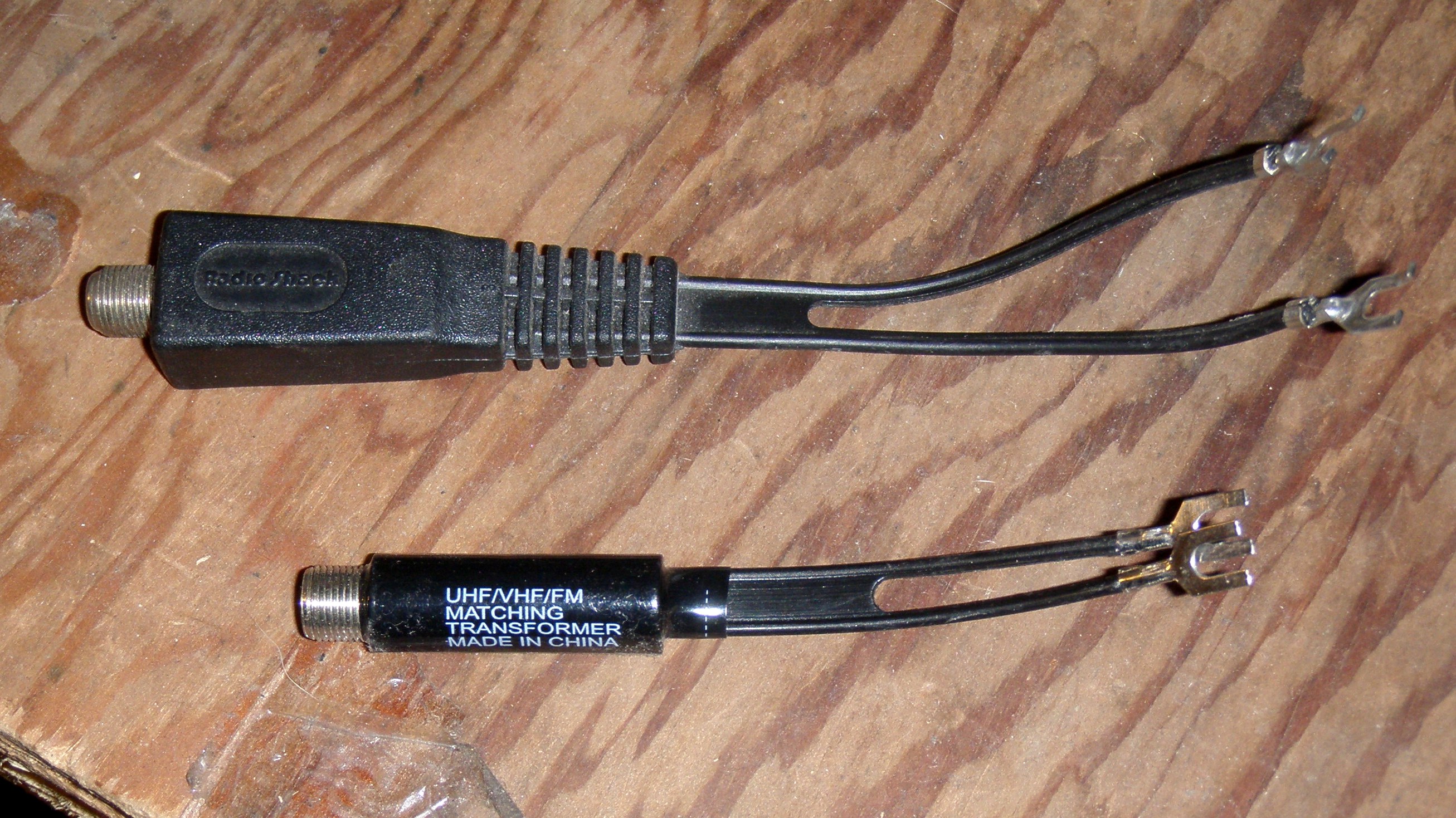
The core is a ferrite toroid or a binocular (two-hole) core, both usually of nickel-zinc ferrite chosen for its high-frequency loss profile; the two-hole binocular shape gives a lot of common-mode impedance in a small volume and is the classic former for 4:1 and 9:1 ununs. The winding is often a length of PTFE-insulated wire pair, or a short run of miniature coax, threaded a few times through the holes. These are the antenna-matching transformers on every ham’s bench: the 1:1 choke balun that feeds a dipole with coax, the 4:1 balun for a folded dipole or a G5RV, the 9:1 unun that lets a 50-ohm rig drive a long random wire (Figure 6). Volume 12’s build projects include winding a 4:1 and a 9:1 on toroids, so the construction detail is deferred there.

8.5 Switch-mode transformers: the ferrite heart of modern power

Every phone charger, laptop brick, LED driver, and computer power supply built in the last four decades contains a small ferrite transformer running not at 50 or 60 hertz but at tens or hundreds of kilohertz. The reason is the design equation that Volume 9 develops in full and Volume 6 previews: the voltage a winding can support is proportional to frequency times core area times flux, so raising the frequency lets the same voltage be handled by a smaller core. A mains transformer for 60 watts is a fist-sized lump of iron; a 60-watt flyback transformer switching at 100 kHz is a ferrite core you can hide under a thumb. Switching converters trade the bulk of iron and copper for the complexity of a fast semiconductor switch and its control loop — a bargain modern electronics takes every time. The core is ferrite (Volume 4) because only ferrite has low enough loss to cycle its flux a hundred thousand times a second without cooking, and the transformer’s design is inseparable from the converter topology it serves.

8.5.1 The flyback: a coupled inductor in disguise

The flyback transformer is the odd one out of the entire dive, because strictly it is not a transformer at all. It is a coupled inductor — an energy-storage device with two windings — and it works in two alternating phases rather than transferring energy continuously (Figure 7). When the primary switch turns on, current ramps up in the primary and the transformer stores energy in its magnetic field, specifically in the air gap deliberately cut into its core (the gap of Volume 4, whose whole purpose is to hold that stored energy without saturating); the secondary diode is reverse-biased and no energy leaves. When the switch turns off, the field collapses, the winding voltages reverse, the secondary diode conducts, and the stored energy is dumped into the output. Primary and secondary therefore never conduct at the same time — the dots are arranged opposed precisely so the secondary is off while the primary charges — and the device is really storing a packet of magnetic charge on one stroke and delivering it on the next.

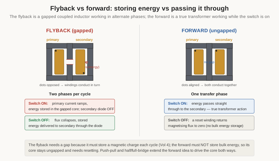
That storage requirement is why a flyback core is gapped and why its designer sizes it by how much energy it can hold, not by how much power it can pass through. The flyback is loved because it is the cheapest way to make an isolated, regulated supply with several outputs from one small transformer and a single switch — hence its universality in low- to medium-power chargers and adapters (a few watts to perhaps 150). Its limitations are the flip side: the core must be big enough to store a whole cycle’s energy, the currents are peaky, and the leakage inductance of that gapped, loosely coupled winding produces a voltage spike at turn-off that must be snubbed. Winding a flyback well — tight primary-to- secondary coupling to minimise leakage, sandwiched or interleaved layers (Volume 5), heavy-build or triple-insulated wire across the isolation barrier — is a craft, and it is where a great deal of switch-mode transformer engineering actually lives.

8.5.2 Forward, push-pull, and bridge: true transformer action

The forward converter and its relatives are proper transformers again. In a forward converter, when the switch turns on the primary voltage appears immediately, scaled by the turns ratio, at the secondary, and energy flows straight through to the output for the whole on-time — true transformer action, no storage stroke. Because it must not store bulk energy, the forward transformer’s core is ungapped; but the magnetising current that inevitably builds during the on-time has to be returned to zero before the next cycle, so the transformer carries a third reset winding (or the circuit uses an active clamp) to demagnetise the core each cycle. Since energy is transferred while the switch conducts rather than stored, the forward converter suits higher powers than the flyback, from tens of watts to a few hundred.

Above that, the push-pull, half-bridge, and full-bridge topologies drive the transformer’s primary alternately in both directions, using the core symmetrically around its B-H loop instead of only in one quadrant. Two switches (push-pull, half-bridge) or four (full-bridge) reverse the primary voltage on successive strokes, so the core’s flux swings positive then negative and its material is used twice as effectively — the route to the highest powers, from a few hundred watts into the kilowatts of server and industrial supplies. These transformers are true, ungapped, tightly coupled devices whose windings must be balanced and symmetric so that neither half of the cycle drives the core off-centre toward saturation, a fault called flux walking that the winder guards against with careful, symmetric layering.

A further refinement worth naming is the resonant converter, of which the LLC half-bridge is the dominant modern form. Here the transformer’s own leakage and magnetising inductances are not parasitics to be minimised but deliberate circuit elements, tuned with a capacitor into a resonant tank so that the switches turn on and off at moments of zero voltage or zero current. That soft switching slashes the switching losses that otherwise rise with frequency, which is precisely what lets LLC designs push into the hundreds of kilohertz and shrink the transformer further — the frequency-versus-size story of Volume 6 taken to its logical end. The flyback, for its part, is frequently built with several secondaries on the one core to produce multiple isolated output rails from a single switch; their voltages track by turns ratio, so a designer trades exact regulation on the minor rails (cross-regulation) for the economy of one transformer, a bargain that suits the many-voltage supplies inside consumer electronics.

8.5.3 Gate-drive and planar transformers

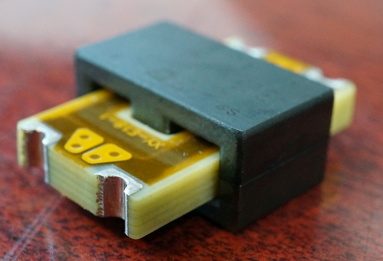
Two specialised switch-mode transformers round out the set. A gate-drive transformer is a tiny, tightly coupled pulse transformer whose only job is to carry the on/off drive signal to the gate of a MOSFET or IGBT while providing galvanic isolation between the low-voltage control circuit and a switch whose source may be flying at hundreds of volts. It transmits information and a little drive energy, not bulk power, and is optimised for fast, clean edges and low leakage rather than efficiency. A planar transformer replaces wound wire entirely with flat copper spirals etched as tracks on a multilayer printed circuit board (or stamped copper foil), clamped between two halves of a low-profile ferrite core (Figure 8). Because the “windings” are photolithographic PCB copper, every unit is identical, the leakage inductance is low and repeatable, the profile is only a few millimetres tall, and the broad flat copper spreads heat well — all of which suit the very high switching frequencies (hundreds of kilohertz into the megahertz) of modern converters, where a wound transformer’s turn-to-turn variability and height become liabilities. The price is that turns are expensive in board layers, isolation across a thin PCB dielectric needs care, and a planar design is locked into its tooling. Planar transformers are the direction of travel for dense, high- frequency power electronics.

8.6 Mapping the zoo onto the rest of the dive

Volumes 7 and 8 together have now named the whole transformer family, and it is worth stepping back to see how it maps onto what follows. The design method of Volume 9 — the 4.44·f·N·B·A electromotive-force equation, volts-per-turn, the window and area-product that size a core, current density and wire gauge, the regulation and temperature-rise budget — applies to every type on the list, but each type stresses a different term. The mains transformer is limited by temperature rise and regulation; the flyback by stored energy and the gap; the RF and balun transformers by bandwidth and common-mode impedance rather than by power at all; the instrument transformer by ratio accuracy and, for protection cores, by the overcurrent at which the iron saturates.

The winding and build volumes (10 to 12) then turn each type into a set of hands. The same coil-winding machines that lay down a mains primary also wind a flyback’s interleaved primary and secondary, thread a secondary onto a CT toroid, and put a few careful turns of coax through a binocular balun core; the difference is in the fixturing, the interleaving, and the insulation discipline, not in the machine. A reader who has followed the type zoo to here can already anticipate which build volume answers which question: a CT or a toroidal power transformer is a threading-and-tensioning job; a flyback or a mains bobbin transformer is a layering-and-insulation job; a balun is a transmission-line-winding job. The types are not really separate technologies so much as one technology — coupled coils on a magnetic core — pushed to different corners of the frequency, power, and accuracy space, and wound to suit.

Table 1 — Mapping the zoo onto the rest of the dive

Type	Typical core	Frequency band	Primary purpose
Current transformer (CT)	Ring of silicon steel or ferrite	50 / 60 Hz	Scale a large current to a safe 5 A (or 1 A) replica
Voltage / potential transformer (VT)	Silicon-steel laminations	50 / 60 Hz	Scale a high voltage to a safe 110 V replica
Tuned IF transformer	Slug-tuned ferrite in a shield can	455 kHz – 45 MHz	Selective coupling and bandpass filtering between IF stages
Broadband RF transformer	NiZn ferrite toroid / binocular	~0.1 – 1000 MHz	Flat impedance matching over many octaves
Balun / unun (transmission-line)	NiZn ferrite toroid / binocular	~1 – 100 MHz	Balance conversion and 1:1 / 4:1 / 9:1 impedance match
Flyback (coupled inductor)	Gapped ferrite (E, RM, pot)	~50 – 500 kHz	Isolated energy storage and release, low-power supplies
Forward / push-pull / bridge	Ungapped ferrite	~50 kHz – 1 MHz	True through-transfer of medium-to-high power
Gate-drive transformer	Small ferrite toroid / EP	switching-rate pulses	Isolated MOSFET / IGBT gate drive
Planar transformer	Low-profile ferrite, PCB windings	hundreds of kHz – MHz	Dense, repeatable, high-frequency power conversion

With the family fully catalogued, the dive turns from what transformers are to how to make one: Volume 9 sizes it, and Volumes 10 through 12 wind it.